In This Page

Introduction

Create Subscriptions

Get Historical Data

Resolutions

Markets

Data Normalization

Wrangle Data

Plot Data

Common Errors

Examples

Datasets

US Equity

Introduction

This page explains how to request, manipulate, and visualize historical US Equity data.

Create Subscriptions

Follow these steps to subscribe to a US Equity security:

Load the assembly files and data types in their own cell.

#load "../Initialize.csx"

Import the data types.

#load "../QuantConnect.csx"
#r "../Microsoft.Data.Analysis.dll"

using QuantConnect;
using QuantConnect.Data;
using QuantConnect.Algorithm;
using QuantConnect.Research;
using QuantConnect.Indicators;
using Microsoft.Data.Analysis;

Create a QuantBook.

Select Language:

var qb = new QuantBook();

qb = QuantBook()

Call the AddEquityadd_equity method with a ticker and then save a reference to the US Equity Symbol.

Select Language:

var spy = qb.AddEquity("SPY").Symbol;
var tlt = qb.AddEquity("TLT").Symbol;

spy = qb.add_equity("SPY").symbol
tlt = qb.add_equity("TLT").symbol

To view the supported assets in the US Equities dataset, see the Data Explorer.

Get Historical Data

You need a subscription before you can request historical data for a security. On the time dimension, you can request an amount of historical data based on a trailing number of bars, a trailing period of time, or a defined period of time. On the security dimension, you can request historical data for a single US Equity, a subset of the US Equities you created subscriptions for in your notebook, or all of the US Equities in your notebook.

Trailing Number of Bars

To get historical data for a number of trailing bars, call the Historyhistory method with the Symbol object(s) and an integer.

Select Language:

// Slice objects
var singleHistorySlice = qb.History(spy, 10);
var subsetHistorySlice = qb.History(new[] {spy, tlt}, 10);
var allHistorySlice = qb.History(10);

// TradeBar objects
var singleHistoryTradeBars = qb.History<TradeBar>(spy, 10);
var subsetHistoryTradeBars = qb.History<TradeBar>(new[] {spy, tlt}, 10);
var allHistoryTradeBars = qb.History<TradeBar>(qb.Securities.Keys, 10);

// QuoteBar objects
var singleHistoryQuoteBars = qb.History<QuoteBar>(spy, 10);
var subsetHistoryQuoteBars = qb.History<QuoteBar>(new[] {spy, tlt}, 10);
var allHistoryQuoteBars = qb.History<QuoteBar>(qb.Securities.Keys, 10);

# DataFrame of trade and quote data
single_history_df = qb.history(spy, 10)
subset_history_df = qb.history([spy, tlt], 10)
all_history_df = qb.history(qb.securities.keys(), 10)

# DataFrame of trade data
single_history_trade_bar_df = qb.history(TradeBar, spy, 10)
subset_history_trade_bar_df = qb.history(TradeBar, [spy, tlt], 10)
all_history_trade_bar_df = qb.history(TradeBar, qb.securities.keys(), 10)

# DataFrame of quote data
single_history_quote_bar_df = qb.history(QuoteBar, spy, 10)
subset_history_quote_bar_df = qb.history(QuoteBar, [spy, tlt], 10)
all_history_quote_bar_df = qb.history(QuoteBar, qb.securities.keys(), 10)

# Slice objects
all_history_slice = qb.history(10)

# TradeBar objects
single_history_trade_bars = qb.history[TradeBar](spy, 10)
subset_history_trade_bars = qb.history[TradeBar]([spy, tlt], 10)
all_history_trade_bars = qb.history[TradeBar](qb.securities.keys(), 10)

# QuoteBar objects
single_history_quote_bars = qb.history[QuoteBar](spy, 10)
subset_history_quote_bars = qb.history[QuoteBar]([spy, tlt], 10)
all_history_quote_bars = qb.history[QuoteBar](qb.securities.keys(), 10)

The preceding calls return the most recent bars, excluding periods of time when the exchange was closed.

Trailing Period of Time

To get historical data for a trailing period of time, call the Historyhistory method with the Symbol object(s) and a TimeSpantimedelta.

Select Language:

// Slice objects
var singleHistorySlice = qb.History(spy, TimeSpan.FromDays(3));
var subsetHistorySlice = qb.History(new[] {spy, tlt}, TimeSpan.FromDays(3));
var allHistorySlice = qb.History(10);

// TradeBar objects
var singleHistoryTradeBars = qb.History<TradeBar>(spy, TimeSpan.FromDays(3));
var subsetHistoryTradeBars = qb.History<TradeBar>(new[] {spy, tlt}, TimeSpan.FromDays(3));
var allHistoryTradeBars = qb.History<TradeBar>(TimeSpan.FromDays(3));

// QuoteBar objects
var singleHistoryQuoteBars = qb.History<QuoteBar>(spy, TimeSpan.FromDays(3), Resolution.Minute);
var subsetHistoryQuoteBars = qb.History<QuoteBar>(new[] {spy, tlt}, TimeSpan.FromDays(3), Resolution.Minute);
var allHistoryQuoteBars = qb.History<QuoteBar>(qb.Securities.Keys, TimeSpan.FromDays(3), Resolution.Minute);

// Tick objects
var singleHistoryTicks = qb.History<Tick>(spy, TimeSpan.FromDays(3), Resolution.Tick);
var subsetHistoryTicks = qb.History<Tick>(new[] {spy, tlt}, TimeSpan.FromDays(3), Resolution.Tick);
var allHistoryTicks = qb.History<Tick>(qb.Securities.Keys, TimeSpan.FromDays(3), Resolution.Tick);

# DataFrame of trade and quote data
single_history_df = qb.history(spy, timedelta(days=3))
subset_history_df = qb.history([spy, tlt], timedelta(days=3))
all_history_df = qb.history(qb.securities.keys(), timedelta(days=3))

# DataFrame of trade data
single_history_trade_bar_df = qb.history(TradeBar, spy, timedelta(days=3))
subset_history_trade_bar_df = qb.history(TradeBar, [spy, tlt], timedelta(days=3))
all_history_trade_bar_df = qb.history(TradeBar, qb.securities.keys(), timedelta(days=3))

# DataFrame of quote data
single_history_quote_bar_df = qb.history(QuoteBar, spy, timedelta(days=3))
subset_history_quote_bar_df = qb.history(QuoteBar, [spy, tlt], timedelta(days=3))
all_history_quote_bar_df = qb.history(QuoteBar, qb.securities.keys(), timedelta(days=3))

# DataFrame of tick data
single_history_tick_df = qb.history(spy, timedelta(days=3), Resolution.TICK)
subset_history_tick_df = qb.history([spy, tlt], timedelta(days=3), Resolution.TICK)
all_history_tick_df = qb.history(qb.securities.keys(), timedelta(days=3), Resolution.TICK)

# Slice objects
all_history_slice = qb.history(timedelta(days=3))

# TradeBar objects
single_history_trade_bars = qb.history[TradeBar](spy, timedelta(days=3))
subset_history_trade_bars = qb.history[TradeBar]([spy, tlt], timedelta(days=3))
all_history_trade_bars = qb.history[TradeBar](qb.securities.keys(), timedelta(days=3))

# QuoteBar objects
single_history_quote_bars = qb.history[QuoteBar](spy, timedelta(days=3), Resolution.MINUTE)
subset_history_quote_bars = qb.history[QuoteBar]([spy, tlt], timedelta(days=3), Resolution.MINUTE)
all_history_quote_bars = qb.history[QuoteBar](qb.securities.keys(), timedelta(days=3), Resolution.MINUTE)

# Tick objects
single_history_ticks = qb.history[Tick](spy, timedelta(days=3), Resolution.TICK)
subset_history_ticks = qb.history[Tick]([spy, tlt], timedelta(days=3), Resolution.TICK)
all_history_ticks = qb.history[Tick](qb.securities.keys(), timedelta(days=3), Resolution.TICK)

The preceding calls return the most recent bars or ticks, excluding periods of time when the exchange was closed.

Defined Period of Time

To get historical data for a specific period of time, call the Historyhistory method with the Symbol object(s), a start DateTimedatetime, and an end DateTimedatetime. The start and end times you provide are based in the notebook time zone.

Select Language:

var startTime = new DateTime(2021, 1, 1);
var endTime = new DateTime(2021, 2, 1);

// Slice objects
var singleHistorySlice = qb.History(spy, startTime, endTime);
var subsetHistorySlice = qb.History(new[] {spy, tlt}, startTime, endTime);
var allHistorySlice = qb.History(qb.Securities.Keys, startTime, endTime);

// TradeBar objects
var singleHistoryTradeBars = qb.History<TradeBar>(spy, startTime, endTime);
var subsetHistoryTradeBars = qb.History<TradeBar>(new[] {spy, tlt}, startTime, endTime);
var allHistoryTradeBars = qb.History<TradeBar>(qb.Securities.Keys, startTime, endTime);

// QuoteBar objects
var singleHistoryQuoteBars = qb.History<QuoteBar>(spy, startTime, endTime, Resolution.Minute);
var subsetHistoryQuoteBars = qb.History<QuoteBar>(new[] {spy, tlt}, startTime, endTime, Resolution.Minute);
var allHistoryQuoteBars = qb.History<QuoteBar>(qb.Securities.Keys, startTime, endTime, Resolution.Minute);

// Tick objects
var singleHistoryTicks = qb.History<Tick>(spy, startTime, endTime, Resolution.Tick);
var subsetHistoryTicks = qb.History<Tick>(new[] {spy, tlt}, startTime, endTime, Resolution.Tick);
var allHistoryTicks = qb.History<Tick>(qb.Securities.Keys, startTime, endTime, Resolution.Tick);

start_time = datetime(2021, 1, 1)
end_time = datetime(2021, 2, 1)

# DataFrame of trade and quote data
single_history_df = qb.history(spy, start_time, end_time)
subset_history_df = qb.history([spy, tlt], start_time, end_time)
all_history_df = qb.history(qb.securities.keys(), start_time, end_time)

# DataFrame of trade data
single_history_trade_bar_df = qb.history(TradeBar, spy, start_time, end_time)
subset_history_trade_bar_df = qb.history(TradeBar, [spy, tlt], start_time, end_time)
all_history_trade_bar_df = qb.history(TradeBar, qb.securities.keys(), start_time, end_time)

# DataFrame of quote data
single_history_quote_bar_df = qb.history(QuoteBar, spy, start_time, end_time)
subset_history_quote_bar_df = qb.history(QuoteBar, [spy, tlt], start_time, end_time)
all_history_quote_bar_df = qb.history(QuoteBar, qb.securities.keys(), start_time, end_time)

# DataFrame of tick data
single_history_tick_df = qb.history(spy, start_time, end_time, Resolution.TICK)
subset_history_tick_df = qb.history([spy, tlt], start_time, end_time, Resolution.TICK)
all_history_tick_df = qb.history(qb.securities.keys(), start_time, end_time, Resolution.TICK)

# TradeBar objects
single_history_trade_bars = qb.history[TradeBar](spy, start_time, end_time)
subset_history_trade_bars = qb.history[TradeBar]([spy, tlt], start_time, end_time)
all_history_trade_bars = qb.history[TradeBar](qb.securities.keys(), start_time, end_time)

# QuoteBar objects
single_history_quote_bars = qb.history[QuoteBar](spy, start_time, end_time, Resolution.MINUTE)
subset_history_quote_bars = qb.history[QuoteBar]([spy, tlt], start_time, end_time, Resolution.MINUTE)
all_history_quote_bars = qb.history[QuoteBar](qb.securities.keys(), start_time, end_time, Resolution.MINUTE)

# Tick objects
single_history_ticks = qb.history[Tick](spy, start_time, end_time, Resolution.TICK)
subset_history_ticks = qb.history[Tick]([spy, tlt], start_time, end_time, Resolution.TICK)
all_history_ticks = qb.history[Tick](qb.securities.keys(), start_time, end_time, Resolution.TICK)

The preceding calls return the bars or ticks that have a timestamp within the defined period of time.

Resolutions

The following table shows the available resolutions and data formats for Equity subscriptions:

Resolution	TradeBar	QuoteBar	Trade Tick	Quote Tick
`TickTICK`
`SecondSECOND`
`MinuteMINUTE`
`HourHOUR`
`DailyDAILY`

Markets

LEAN groups all of the US Equity exchanges under Market.USA.

Data Normalization

The data normalization mode defines how historical data is adjusted for corporate actions. By default, LEAN adjusts US Equity data for splits and dividends to produce a smooth price curve, but the following data normalization modes are available:

If you use AdjustedADJUSTED, SplitAdjustedSPLIT_ADJUSTED, or TotalReturnTOTAL_RETURN, we use the entire split and dividend history to adjust historical prices. This process ensures you get the same adjusted prices, regardless of the QuantBook time. If you use ScaledRawSCALED_RAW, we use the split and dividend history before the QuantBook's EndDate to adjust historical prices.

To set the data normalization mode for a security, pass a dataNormalizationModedata_normalization_mode argument to the AddEquityadd_equity method.

Select Language:

var spy = qbAddEquity("SPY", dataNormalizationMode: DataNormalizationMode.Raw).Symbol;

spy = qb.add_equity("SPY", data_normalization_mode=DataNormalizationMode.RAW).symbol

When you request historical data, the Historyhistory method uses the data normalization of your security subscription. To get historical data with a different data normalization, pass a dataNormalizationModedata_normalization_mode argument to the Historyhistory method.

Select Language:

var history = qb.History(qb.Securities.Keys, qb.Time-TimeSpan.FromDays(10), qb.Time, dataNormalizationMode: DataNormalizationMode.SplitAdjusted);

history = qb.history(qb.securities.keys(), qb.time-timedelta(days=10), qb.time, dataNormalizationMode=DataNormalizationMode.SPLIT_ADJUSTED)

Wrangle Data

You need some historical data to perform wrangling operations. The process to manipulate the historical data depends on its data type. To display pandas objects, run a cell in a notebook with the pandas object as the last line. To display other data formats, call the print method.

You need some historical data to perform wrangling operations. Use LINQ to wrangle the data and then call the Console.WriteLine method in a Jupyter Notebook to display the data. The process to manipulate the historical data depends on its data type.

DataFrame Objects

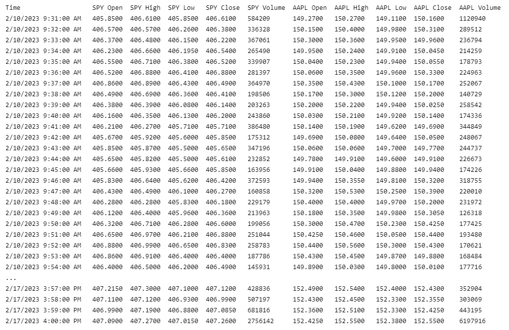
If the Historyhistory method returns a DataFrame, the first level of the DataFrame index is the encoded Equity Symbol and the second level is the EndTimeend_time of the data sample. The columns of the DataFrame are the data properties.

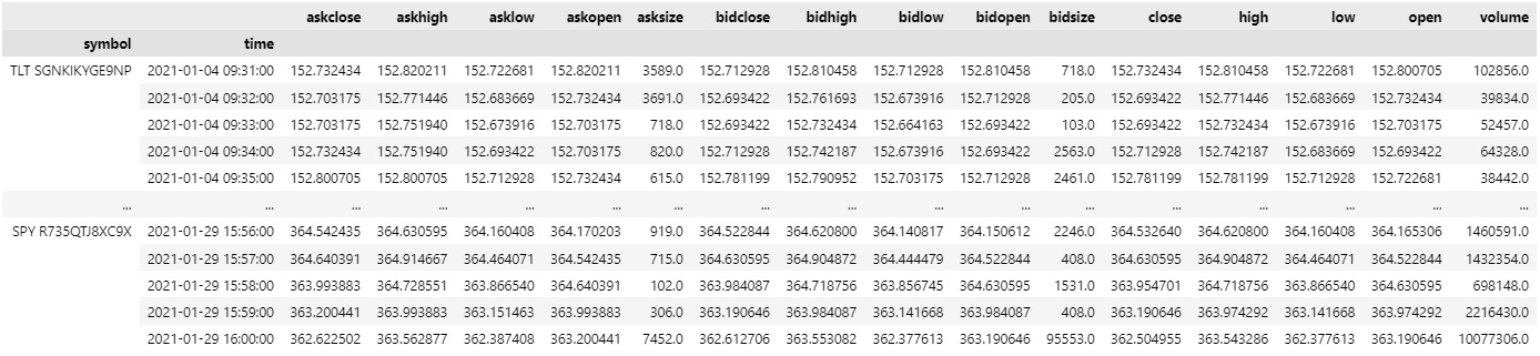
To select the historical data of a single Equity, index the loc property of the DataFrame with the Equity Symbol.

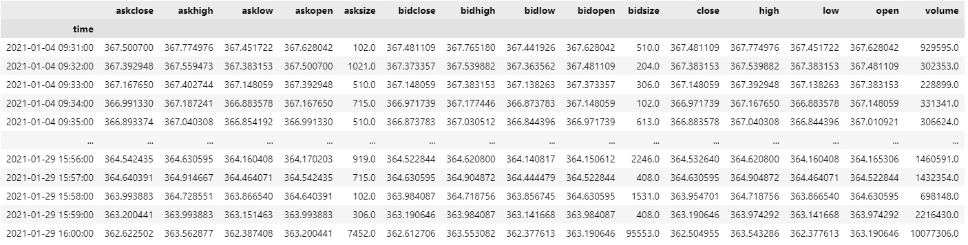
all_history_df.loc[spy]  # or all_history_df.loc['SPY']

To select a column of the DataFrame, index it with the column name.

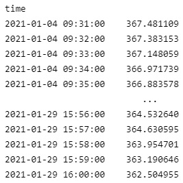
all_history_df.loc[spy]['close']

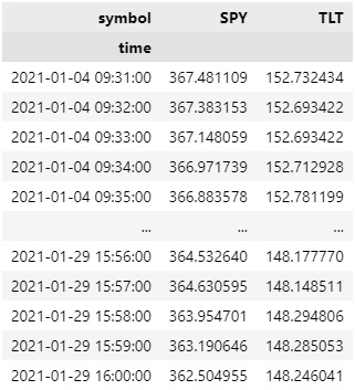
If you request historical data for multiple Equities, you can transform the DataFrame so that it's a time series of close values for all of the Equities. To transform the DataFrame, select the column you want to display for each Equity and then call the unstack method.

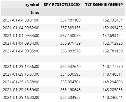
all_history_df['close'].unstack(level=0)

The DataFrame is transformed so that the column indices are the Symbol of each Equity and each row contains the close value.

If you prefer to display the ticker of each Symbol instead of the string representation of the SecurityIdentifier, follow these steps:

Create a dictionary where the keys are the string representations of each SecurityIdentifier and the values are the ticker.

tickers_by_id = {str(x.id): x.value for x in qb.securities.keys}

Get the values of the symbol level of the DataFrame index and create a list of tickers.

tickers = set([tickers_by_id[x] for x in all_history_df.index.get_level_values('symbol')])

Set the values of the symbol level of the DataFrame index to the list of tickers.

all_history_df.index.set_levels(tickers, 'symbol', inplace=True)

The new DataFrame is keyed by the ticker.

all_history_df.loc[spy.value]  # or all_history_df.loc["SPY"]

After the index renaming, the unstacked DataFrame has the following format:

Historical data dataframe of selected attribute by symbols

using Microsoft.Data.Analysis; 

var columns = new DataFrameColumn[] {
    new PrimitiveDataFrameColumn("Time", history.Select(x => x[spy].EndTime)),
    new DecimalDataFrameColumn("SPY Open", history.Select(x => x[spy].Open)),
    new DecimalDataFrameColumn("SPY High", history.Select(x => x[spy].High)),
    new DecimalDataFrameColumn("SPY Low", history.Select(x => x[spy].Low)),
    new DecimalDataFrameColumn("SPY Close", history.Select(x => x[spy].Close))
};
var df = new DataFrame(columns);
df

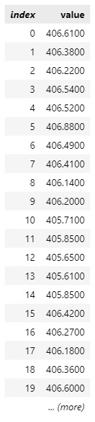
df["SPY close"]

Slice Objects

If the Historyhistory method returns Slice objects, iterate through the Slice objects to get each one. The Slice objects may not have data for all of your Equity subscriptions. To avoid issues, check if the Slice contains data for your Equity before you index it with the Equity Symbol.

Select Language:

foreach (var slice in allHistorySlice) {
    if (slice.Bars.ContainsKey(spy))
    {
        var tradeBar = slice.Bars[spy];
    }
    if (slice.QuoteBars.ContainsKey(spy))
    {
        var quoteBar = slice.QuoteBars[spy];
    }
}

for slice in all_history_slice:
        if slice.bars.contains_key(spy):
        trade_bar = slice.bars[spy]
    if slice.quote_bars.contains_key(spy):
        quote_bar = slice.quote_bars[spy]

You can also iterate through each TradeBar and QuoteBar in the Slice.

Select Language:

foreach (var slice in allHistorySlice)
{
    foreach (var kvp in slice.Bars)
    {
        var symbol = kvp.Key;
        var tradeBar = kvp.Value;
    }
    foreach (var kvp in slice.QuoteBars)
    {
        var symbol = kvp.Key;
        var quoteBar = kvp.Value;
    }
}

for slice in all_history_slice:
    for kvp in slice.bars:
        symbol = kvp.key
        trade_bar = kvp.value
    for kvp in slice.quote_bars:
        symbol = kvp.key
        quote_bar = kvp.value

You can also use LINQ to select each TradeBar in the Slice for a given Symbol.

var tradeBars = allHistorySlice.Where(slice => slice.Bars.ContainsKey(spy)).Select(slice => slice.Bars[spy]);

TradeBar Objects

If the Historyhistory method returns TradeBar objects, iterate through the TradeBar objects to get each one.

Select Language:

foreach (var tradeBar in singleHistoryTradeBars)
{
    Console.WriteLine(tradeBar);
}

for trade_bar in single_history_trade_bars:
    print(trade_bar)

If the Historyhistory method returns TradeBars, iterate through the TradeBars to get the TradeBar of each Equity. The TradeBars may not have data for all of your Equity subscriptions. To avoid issues, check if the TradeBars object contains data for your security before you index it with the Equity Symbol.

Select Language:

foreach (var tradeBars in allHistoryTradeBars)
{
    if (tradeBars.ContainsKey(spy))
    {
        var tradeBar = tradeBars[spy];
    }
}

for trade_bars in all_history_trade_bars:
    if trade_bars.contains_key(spy):
        trade_bar = trade_bars[spy]

You can also iterate through each of the TradeBars.

Select Language:

foreach (var tradeBars in allHistoryTradeBars)
{
    foreach (var kvp in tradeBars)
    {
        var symbol = kvp.Key;
        var tradeBar = kvp.Value;
    }
}

for trade_bars in all_history_trade_bars:
    for kvp in trade_bars:
        symbol = kvp.Key
        trade_bar = kvp.Value

QuoteBar Objects

If the Historyhistory method returns QuoteBar objects, iterate through the QuoteBar objects to get each one.

Select Language:

foreach (var quoteBar in singleHistoryQuoteBars)
{
    Console.WriteLine(quoteBar);
}

for quote_bar in single_history_quote_bars:
    print(quote_bar)

If the Historyhistory method returns QuoteBars, iterate through the QuoteBars to get the QuoteBar of each Equity. The QuoteBars may not have data for all of your Equity subscriptions. To avoid issues, check if the QuoteBars object contains data for your security before you index it with the Equity Symbol.

Select Language:

foreach (var quoteBars in allHistoryQuoteBars)
{
    if (quoteBars.ContainsKey(spy))
    {
        var quoteBar = quoteBars[spy];
    }
}

for quote_bars in all_history_quote_bars:
    if quote_bars.contains_key(spy):
        quote_bar = quote_bars[spy]

You can also iterate through each of the QuoteBars.

Select Language:

foreach (var quoteBars in allHistoryQuoteBars)
{
    foreach (var kvp in quoteBars)
    {
        var symbol = kvp.Key;
        var quoteBar = kvp.Value;
    }
}

for quote_bars in all_history_quote_bars:
    for kvp in quote_bars:
        symbol = kvp.key
        quote_bar = kvp.value

Tick Objects

If the Historyhistory method returns TickTICK objects, iterate through the TickTICK objects to get each one.

Select Language:

foreach (var tick in singleHistoryTicks)
{
    Console.WriteLine(tick);
}

for tick in single_history_ticks:
    print(tick)

If the Historyhistory method returns Ticks, iterate through the Ticks to get the TickTICK of each Equity. The Ticks may not have data for all of your Equity subscriptions. To avoid issues, check if the Ticks object contains data for your security before you index it with the Equity Symbol.

Select Language:

foreach (var ticks in allHistoryTicks)
{
    if (ticks.ContainsKey(spy))
    {
        var tick = ticks[spy];
    }
}

for ticks in all_history_ticks:
    if ticks.contains_key(spy):
        ticks = ticks[spy]

You can also iterate through each of the Ticks.

Select Language:

foreach (var ticks in allHistoryTicks)
{
    foreach (var kvp in ticks)
    {
        var symbol = kvp.Key;
        var tick = kvp.Value;
    }
}

for ticks in all_history_ticks:
    for kvp in ticks:
        symbol = kvp.key
        tick = kvp.value

The Ticks objects only contain the last tick of each security for that particular timeslice

Plot Data

You need some historical Equity data to produce plots. You can use many of the supported plotting librariesPlot.NET package to visualize data in various formats. For example, you can plot candlestick and line charts.

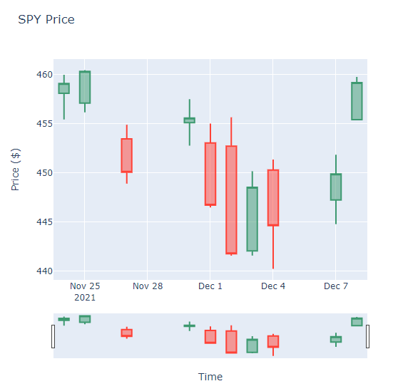
Candlestick Chart

Follow these steps to plot candlestick charts:

Get some historical data.

Select Language:

history = qb.history(spy, datetime(2021, 11, 23), datetime(2021, 12, 8), Resolution.DAILY).loc[spy]

var history = qb.History<TradeBar>(spy, new DateTime(2021, 11, 23), new DateTime(2021, 12, 8), Resolution.Daily);

Import the plotlyPlot.NET library.

Select Language:

import plotly.graph_objects as go

#r "../Plotly.NET.dll"
using Plotly.NET;
using Plotly.NET.LayoutObjects;

Create a Candlestick chart.

Select Language:

candlestick = go.Candlestick(x=history.index,
                             open=history['open'],
                             high=history['high'],
                             low=history['low'],
                             close=history['close'])

var chart = Chart2D.Chart.Candlestick<decimal, decimal, decimal, decimal, DateTime, string>(
    history.Select(x => x.Open),
    history.Select(x => x.High),
    history.Select(x => x.Low),
    history.Select(x => x.Close),
    history.Select(x => x.EndTime)
);

Create a Layout.

Select Language:

layout = go.Layout(title=go.layout.Title(text='SPY OHLC'),
                   xaxis_title='Date',
                   yaxis_title='Price',
                   xaxis_rangeslider_visible=False)

LinearAxis xAxis = new LinearAxis();
xAxis.SetValue("title", "Time");
LinearAxis yAxis = new LinearAxis();
yAxis.SetValue("title", "Price ($)");
Title title = Title.init("SPY Price");

Layout layout = new Layout();
layout.SetValue("xaxis", xAxis);
layout.SetValue("yaxis", yAxis);
layout.SetValue("title", title);

Create the Figure.
Assign the Layout to the chart.

Select Language:

fig = go.Figure(data=[candlestick], layout=layout)

chart.WithLayout(layout);

Show the plot.

Select Language:

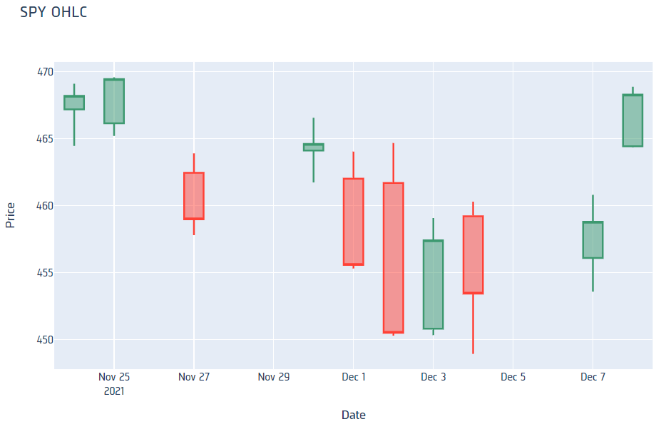
fig.show()

HTML(GenericChart.toChartHTML(chart))

Candlestick charts display the open, high, low, and close prices of the security.

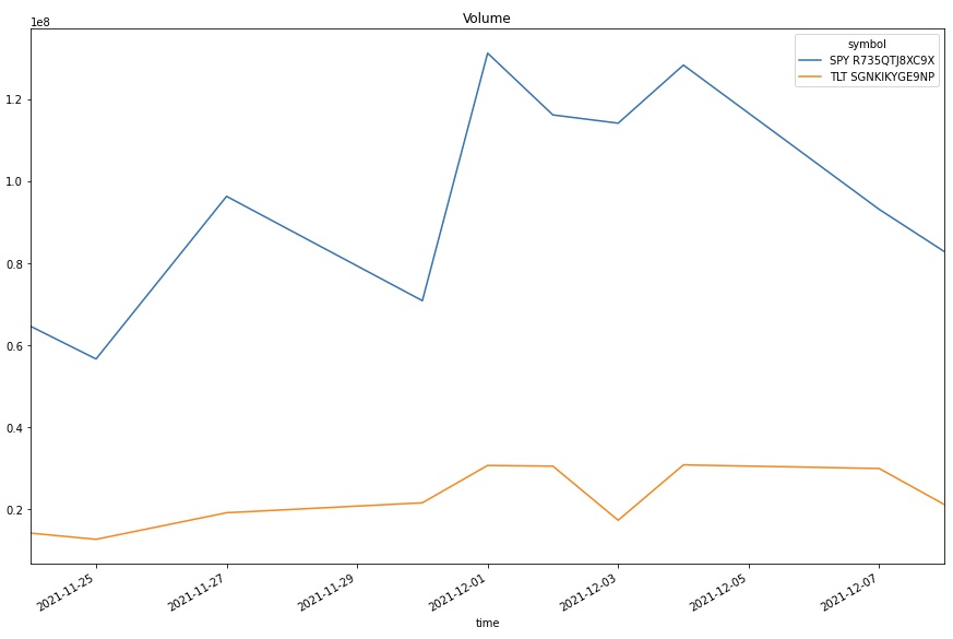
Line Chart

Follow these steps to plot line charts using built-in methodsPlotly.NET package:

Get some historical data.

Select Language:

history = qb.history([spy, tlt], datetime(2021, 11, 23), datetime(2021, 12, 8), Resolution.DAILY)

var history = qb.History<TradeBar>(new [] {spy, tlt}, new DateTime(2021, 11, 23), new DateTime(2021, 12, 8), Resolution.Daily);

Select the data to plot.

Select Language:

volume = history['volume'].unstack(level=0)

var spy = history.Select(x => x["SPY"]);

Call the plot method on the pandas object.
Create a Line chart.

Select Language:

volume.plot(title="Volume", figsize=(15, 10))

var chart = Chart2D.Chart.Line<DateTime, decimal, string>(
    spy.Select(x => x.EndTime),
    spy.Select(x => x.Volume)
);

Create a Layout.

LinearAxis xAxis = new LinearAxis();
xAxis.SetValue("title", "Time");
LinearAxis yAxis = new LinearAxis();
yAxis.SetValue("title", "Volume");
Title title = Title.init("SPY Volume");

Layout layout = new Layout();
layout.SetValue("xaxis", xAxis);
layout.SetValue("yaxis", yAxis);
layout.SetValue("title", title);

Assign the Layout to the chart.

chart.WithLayout(layout);

Show the plot.

Select Language:

plt.show()

HTML(GenericChart.toChartHTML(chart))

Line charts display the value of the property you selected in a time series.

Common Errors

Some factor files have INF split values, which indicate that the stock has so many splits that prices can't be calculated with correct numerical precision. To allow history requests with these symbols, we need to move the starting date forward when reading the data or use raw data normalization. If there are numerical precision errors in the factor files for a security in your history request, LEAN throws the following error:

"Warning: when performing history requests, the start date will be adjusted if there are numerical precision errors in the factor files."

Examples

The following examples demonstrate some common practices for applying the US Equity dataset.

Example 1: 5-Minute Candlestick Plot

The following example studies the candlestick pattern of the SPY. To study the short term pattern, we consolidate the data into 5 minute bars and plot the 5-minute candlestick plot.

Select Language:

// Load the required assembly files and data types in a separate cell.
#load "../Initialize.csx"

#load "../QuantConnect.csx"
using System;
using QuantConnect;
using QuantConnect.Data;
using QuantConnect.Data.Market;
using QuantConnect.Data.Consolidators;
using QuantConnect.Indicators;
using QuantConnect.Algorithm;
using QuantConnect.Research;
using QuantConnect.Securities;

// Import Plotly for plotting.
#r "../Plotly.NET.dll"
using Plotly.NET;
using Plotly.NET.LayoutObjects;

// Create a QuantBook.
var qb = new QuantBook();

// Request the SPY historical data.
var spy = qb.AddEquity("SPY");
var history = qb.History<TradeBar>(spy.Symbol, 
    start: qb.Time - TimeSpan.FromDays(182),
    end: qb.Time,
    resolution: Resolution.Minute);

// Set up a consolidator and a RollingWindow to save the data
var consolidator = new TradeBarConsolidator(TimeSpan.FromMinutes(5));
var window = new RollingWindow<TradeBar>(10000);

// Attach a consolidation handler method that saves the consolidated bars in the RollingWindow
consolidator.DataConsolidated += (sender, consolidated) =>
{
    window.Add(consolidated);
};

// Iterate the historical market data and feed each bar into the consolidator
foreach(var bar in history)
{
    consolidator.Update(bar);
}

// Crete the Candlestick chart using the 5-minute windows.
var chart = Chart2D.Chart.Candlestick<decimal, decimal, decimal, decimal, DateTime, string>(
    window.Select(x => x.Open),
    window.Select(x => x.High),
    window.Select(x => x.Low),
    window.Select(x => x.Close),
    window.Select(x => x.EndTime)
);
// Create a Layout as the plot settings.
LinearAxis xAxis = new LinearAxis();
xAxis.SetValue("title", "Time");
LinearAxis yAxis = new LinearAxis();
yAxis.SetValue("title", "Price ($)");
Title title = Title.init($"{spy.Symbol} Price");

Layout layout = new Layout();
layout.SetValue("xaxis", xAxis);
layout.SetValue("yaxis", yAxis);
layout.SetValue("title", title);
// Assign the Layout to the chart.
chart.WithLayout(layout);
// Display the plot.
HTML(GenericChart.toChartHTML(chart))

# Import plotly library for plotting.
import plotly.graph_objects as go

# Create a QuantBook
qb = QuantBook()

# Request SPY's historical data.
spy = qb.add_equity("SPY")
history = qb.history(spy.symbol, 
    start=qb.time - timedelta(days=182), 
    end=qb.time, 
    resolution=Resolution.MINUTE)

# Drop level 0 index (Symbol index) from the DataFrame
history = history.droplevel([0])

# Select the required columns to obtain the 5-minute OHLC data.
history = history[["open", "high", "low", "close"]].resample("5T").agg({
    "open": "first",
    "high": "max",
    "low": "min",
    "close": "last"
})

# Crete the Candlestick chart using the 5-minute windows.
candlestick = go.Candlestick(x=history.index,
                             open=history['open'],
                             high=history['high'],
                             low=history['low'],
                             close=history['close'])
# Create a Layout as the plot settings.
layout = go.Layout(title=go.layout.Title(text=f'{spy.symbol} OHLC'),
                   xaxis_title='Date',
                   yaxis_title='Price',
                   xaxis_rangeslider_visible=False)
# Create the Figure.
fig = go.Figure(data=[candlestick], layout=layout)
# Display the plot.
fig.show()

You can also see our Videos. You can also get in touch with us via Discord.

Did you find this page helpful?

Contribute to the documentation:

SIGN IN

Browse

Cloud Platform

Writing Algorithms

Research Environment

▶Key Concepts

Initialization

▶Datasets

▶Charting

Universes

▶Indicators

Object Store

▶Machine Learning

Debugging

▶Meta Analysis

▶Applying Research

Local Platform

LEAN CLI

LEAN Engine

Hello

Datasets

US Equity

Introduction

Create Subscriptions

Get Historical Data

Trailing Number of Bars

Trailing Period of Time

Defined Period of Time

Resolutions

Markets

Data Normalization

Wrangle Data

DataFrame Objects

Slice Objects

TradeBar Objects

QuoteBar Objects

Tick Objects

Plot Data

Candlestick Chart

Line Chart

Common Errors

Examples

Example 1: 5-Minute Candlestick Plot

▶
Key Concepts

▶
Datasets

▶
Charting

▶
Indicators

▶
Machine Learning

▶
Meta Analysis

▶
Applying Research