Index Options

Follow these steps to subscribe to an Index Option universe:

1. Load the assembly files and data types in their own cell.

#load "../Initialize.csx"

2. Import the data types.

#load "../QuantConnect.csx"
#r "../Microsoft.Data.Analysis.dll"

using QuantConnect;
using QuantConnect.Data;
using QuantConnect.Algorithm;
using QuantConnect.Research;
using QuantConnect.Indicators;
using QuantConnect.Securities.Index;
using QuantConnect.Securities.IndexOption;
using QuantConnect.Data.UniverseSelection;
using Microsoft.Data.Analysis;

3. Create a QuantBook.

var qb = new QuantBook();

qb = QuantBook()

4. Add the underlying Index.

var indexSymbol = qb.AddIndex("SPX", Resolution.Minute).Symbol;

index_symbol = qb.add_index("SPX", Resolution.MINUTE).symbol

To view the available Indices, see Supported Assets.

If you do not pass a resolution argument, Resolution.MinuteResolution.MINUTE is used by default.


5. Call the AddIndexOptionadd_index_option method with the underlying Index Symbol and, if you want non-standard Index Options, the target Option ticker.

var option = qb.AddIndexOption(indexSymbol);

option = qb.add_index_option(index_symbol)

The contract filter determines which Index Option contracts are in your universe each trading day. The default filter selects the contracts with the following characteristics:

• Standard type (exclude weeklys)
• Within 1 strike price of the underlying asset price
• Expire within 35 days

To change the filter, call the SetFilterset_filter method.

// Set the contract filter to select contracts that have the strike price 
// within 1 strike level and expire within 90 days.
option.SetFilter(-1, 1, 0, 90);

# Set the contract filter to select contracts that have the strike price 
# within 1 strike level and expire within 90 days.
option.set_filter(-1, 1, 0, 90)

To get the prices and volumes for all of the Index Option contracts that pass your filter during a specific period of time, call the OptionHistoryoption_history method with the underlying Index Symbol object, a start DateTimedatetime, and an end DateTimedatetime.

option_history = qb.option_history(
    index_symbol, datetime(2024, 1, 1), datetime(2024, 1, 5), Resolution.MINUTE, 
    fill_forward=False, extended_market_hours=False
)

var optionHistory = qb.OptionHistory(
    indexSymbol, new DateTime(2024, 1, 1), new DateTime(2024, 1, 5), Resolution.Minute,
    fillForward: false, extendedMarketHours: false
);

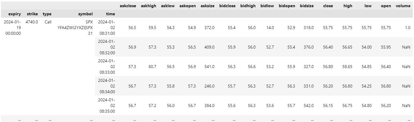
To convert the OptionHistory object to a DataFrame that contains the trade and quote information of each contract and the underlying, use the data_frame property.

option_history.data_frame

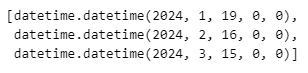
To get the expiration dates of all the contracts in an OptionHistory object, call the GetExpiryDatesget_expiry_dates method.

option_history.get_expiry_dates()

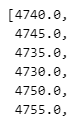
To get the strike prices of all the contracts in an OptionHistory object, call the GetStrikesget_strikes method.

option_history.get_strikes()

To get daily data on all the tradable contracts for a given date, call the History<OptionUniverse>history method with the canoncial Option Symbol, a start date, and an end date. This method returns the entire Option chain for each trading day, not the subset of contracts that pass your universe filter. The daily Option chains contain the prices, volume, open interest, implied volaility, and Greeks of each contract.

# DataFrame format
history_df = qb.history(option.symbol, datetime(2024, 1, 1), datetime(2024, 1, 5), flatten=True)

# OptionUniverse objects
history = qb.history[OptionUniverse](option.symbol, datetime(2024, 1, 1), datetime(2024, 1, 5))
for chain in history:
    end_time = chain.end_time
    filtered_chain = [contract for contract in chain if contract.greeks.delta > 0.3]
    for contract in filtered_chain:
        price = contract.price
        iv = contract.implied_volatility

var history = qb.History<OptionUniverse>(option.Symbol, new DateTime(2024, 1, 1), new DateTime(2024, 1, 5));
foreach (var chain in history)
{
    var endTime = chain.EndTime;
    var filteredChain = chain.Data
        .Select(contract => contract as OptionUniverse)
        .Where(contract => contract.Greeks.Delta > 0.3m);
    foreach (var contract in filteredChain)
    {
        var price = contract.Price;
        var iv = contract.ImpliedVolatility;
    }
}

The method represents each contract with an OptionUniverse object, which have the following properties: