In This Page

Introduction

Create Hypothesis

Import Libraries

Get Historical Data

Prepare Data

Test Hypothesis

Set Up Algorithm

Examples

Applying Research

Uncorrelated Assets

Introduction

This page explains how to you can use the Research Environment to develop and test a Uncorrelated Assets hypothesis, then put the hypothesis in production.

Create Hypothesis

According to Modern Portfolio Thoery, asset combinations with negative or very low correlation could have lower total portfolio variance given the same level of return. Thus, uncorrelated assets allows you to find a portfolio that will, theoretically, be more diversified and resilient to extreme market events. We're testing this statement in real life scenario, while hypothesizing a portfolio with uncorrelated assets could be a consistent portfolio. In this example, we'll compare the performance of 5-least-correlated-asset portfolio (proposed) and 5-most-correlated-asset portfolio (benchmark), both equal weighting.

Import Libraries

We'll need to import libraries to help with data processing and visualization. Import numpy and matplotlib libraries by the following:

Select Language:

#load "../Initialize.csx"
#load "../QuantConnect.csx"

using QuantConnect;
using QuantConnect.Data;
using QuantConnect.Data.Market;
using QuantConnect.Algorithm;
using QuantConnect.Research;
using System;
using System.Linq;
using Accord.Statistics;

import numpy as np
from matplotlib import pyplot as plt

Get Historical Data

To begin, we retrieve historical data for researching.

Instantiate a QuantBook.

Select Language:

var qb = new QuantBook();

qb = QuantBook()

Select the desired tickers for research.

Select Language:

var assets = new List<string>() {"SHY", "TLT", "SHV", "TLH", "EDV", "BIL",
                  "SPTL", "TBT", "TMF", "TMV", "TBF", "VGSH", "VGIT",
                  "VGLT", "SCHO", "SCHR", "SPTS", "GOVT"};

assets = ["SHY", "TLT", "SHV", "TLH", "EDV", "BIL",
          "SPTL", "TBT", "TMF", "TMV", "TBF", "VGSH", "VGIT",
          "VGLT", "SCHO", "SCHR", "SPTS", "GOVT"]

Call the AddEquityadd_equity method with the tickers, and their corresponding resolution.

Select Language:

foreach(var ticker in assets){
    qb.AddEquity(ticker, Resolution.Minute);
}

for i in range(len(assets)):
    qb.add_equity(assets[i],Resolution.MINUTE)

If you do not pass a resolution argument, Resolution.MinuteResolution.MINUTE is used by default.

Call the Historyhistory method with qb.Securities.Keysqb.securities.keys for all tickers, time argument(s), and resolution to request historical data for the symbol.

Select Language:

var history = qb.History(qb.Securities.Keys, new DateTime(2021, 1, 1), new DateTime(2021, 12, 31), Resolution.Daily);

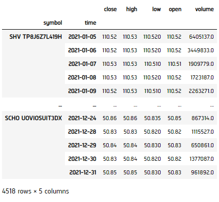
history = qb.history(qb.securities.keys(), datetime(2021, 1, 1), datetime(2021, 12, 31), Resolution.DAILY)

Prepare Data

We'll have to process our data to get their correlation and select the least and most related ones.

Extract daily return for each Symbol from Slice data.
Select the close column and then call the unstack method, then call pct_change to compute the daily return.

Select Language:

var returns = new Dictionary<string, List<Double>>();
var last = new Dictionary<string, Double>();
foreach(var slice in history){
    foreach(var symbol in slice.Bars.Keys){
        if(!returns.ContainsKey(symbol)){
            returns.Add(symbol, new List<Double>());
            last.Add(symbol, (Double)slice.Bars[symbol].Close);
        }
        var change = (Double) ((Double)slice.Bars[symbol].Close - last[symbol])/last[symbol];
        last[symbol] = (Double)slice.Bars[symbol].Close;
        returns[symbol].Add(change);
    }    
}

returns = history['close'].unstack(level=0).pct_change().iloc[1:]

Extract daily return for each Symbol from Slice data.

double[,] ret = new double[returns.Values.ElementAt(0).Count - 1, assets.Count];
int k = 0;
foreach(var kvp in returns)
{
    var symbol = kvp.Key;
    for(int i=0; i < returns[symbol].Count - 1; i++)
    {
        ret[i, k] = returns[symbol][i + 1];
    }
    k++;
}

Write a function to obtain the least and most correlated 5 assets.

Select Language:

public Dictionary<string, Double> GetCorrelations(double[,] returns){
    // Get correlation matrix
    var corrMatrix = Measures.Correlation(ret);
    
    // Find the absolute sum correlation of the assets
    var correlations = new Dictionary<string, Double>();
    for(int i=0; i < corrMatrix.GetLength(0); i++)
    {
        var symbol = assets[i];
        if(!correlations.ContainsKey(symbol)){
            correlations.Add(symbol, 0);
        }
        for (int j=0; j < corrMatrix.GetLength(1); j++)
        {
            var value_ = corrMatrix[i, j];
            correlations[symbol] += value_ >= 0 ? value_ : -value_;
        }
    }
    
    return correlations;
}

var corr = GetCorrelations(ret);
var selected = corr.OrderBy(x => x.Value).Take(5);
var benchmark = corr.OrderBy(x => x.Value).TakeLast(5);

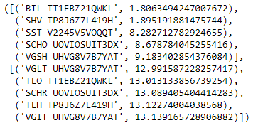
def get_uncorrelated_assets(returns, num_assets):
    # Get correlation
    correlation = returns.corr()
    
    # Find assets with lowest and highest absolute sum correlation
    selected = []
    for index, row in correlation.iteritems():
        corr_rank = row.abs().sum()
        selected.append((index, corr_rank))

    # Sort and take the top num_assets
    sort_ = sorted(selected, key = lambda x: x[1])
    uncorrelated = sort_[:num_assets]
    correlated = sort_[-num_assets:]
    
    return uncorrelated, correlated

selected, benchmark = get_uncorrelated_assets(returns, 5)

Test Hypothesis

To test the hypothesis: Our desired outcome would be a consistent and low fluctuation equity curve should be seen, as compared with benchmark.

Construct a equal weighting portfolio for the 5-uncorrelated-asset-portfolio and the 5-correlated-asset-portfolio (benchmark).

Select Language:

double[,] portRet = new double[returns.Values.ElementAt(0).Count, 5];
int j = 0;
foreach(var kvp in selected){
    var symbol = kvp.Key;
    for(int i=0; i < returns[symbol].Count; i++)
    {
        portRet[i, j] = returns[symbol][i] / 5;
    }
    j++;
}

double[,] benchRet = new double[returns.Values.ElementAt(0).Count, 5];
j = 0;
foreach(var kvp in benchmark){
    var symbol = kvp.Key;
    for(int i=0; i < returns[symbol].Count; i++)
    {
        benchRet[i, j] = returns[symbol][i] / 5;
    }
    j++;
}

port_ret = returns[[x[0] for x in selected]] / 5
bench_ret = returns[[x[0] for x in benchmark]] / 5

Get the Equity Return for both portfolios.
Call cumprod to get the cumulative return.

Select Language:

var totalValue = new List<double>{1.0};
var dailySum = 0.0;
for(int i=0; i < portRet.GetLength(0); i++)
{
    totalValue.Add(totalValue.Last() * (1 + dailySum));
    dailySum = 0.0;
    for (int j=0; j < portRet.GetLength(1); j++)
    {
        if (double.IsFinite(portRet[i, j]))
        {
            dailySum += portRet[i, j];
        }
    }
}

var totalValueBench = new List<double>{1.0};
var dailySumBench = 0.0;
for(int i=0; i < benchRet.GetLength(0); i++)
{
    totalValueBench.Add(totalValueBench.Last() * (1 + dailySumBench));
    dailySumBench = 0.0;
    for (int j=0; j < benchRet.GetLength(1); j++)
    {
        if (double.IsFinite(benchRet[i, j]))
        {
            dailySumBench += benchRet[i, j];
        }
    }
}

total_ret = (np.sum(port_ret, axis=1) + 1).cumprod()
total_ret_bench = (np.sum(bench_ret, axis=1) + 1).cumprod()

Calculate the variance of the 2 portfolios.

var returnPort = new List<double>();
previous = 0.0;
for(int i=0; i < totalValue.Count; i++)
{
    var current = totalValue[i];
    returnPort.Add((current - previous) / previous);
    previous = current;
}
var varPort = Math.Sqrt(returnPort.Skip(1).Average(v=>Math.Pow(v-returnPort.Skip(1).Average(),2)));

var returnBench = new List<double>();
previous = 0.0;
for(int i=0; i < totalValueBench.Count; i++)
{
    var current = totalValueBench[i];
    returnBench.Add((current - previous) / previous);
    previous = current;
}
var varBench = Math.Sqrt(returnBench.Skip(1).Average(v=>Math.Pow(v-returnBench.Skip(1).Average(),2)));

Print the result.
Plot the result.

Select Language:

Console.WriteLine("Portfolio Return: {0}, Variance: {1}", (totalValue.Last() - totalValue.First())/totalValue.First(), varPort);
Console.WriteLine("Benchmark Return: {0}, Variance: {1}", (totalValueBench.Last() - totalValueBench.First())/totalValueBench.First(), varBench);

plt.figure(figsize=(15, 10))
total_ret.plot(label='Proposed')
total_ret_bench.plot(label='Benchmark')
plt.title('Equity Curve')
plt.legend()
plt.show()

-image

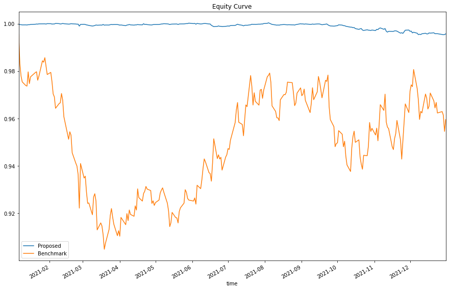
We can clearly see from the results, the proposed uncorrelated-asset-portfolio has a lower variance/fluctuation, thus more consistent than the benchmark. This proven our hypothesis.

Set Up Algorithm

Once we are confident in our hypothesis, we can export this code into backtesting. One way to accomodate this model into research is to create a scheduled event which uses our model to pick stocks and goes long.

Select Language:

private List<string> _asset = new List<string>{"SHY", "TLT", "IEI", "SHV", "TLH", "EDV", "BIL",
        "SPTL", "TBT", "TMF", "TMV", "TBF", "VGSH", "VGIT",
        "VGLT", "SCHO", "SCHR", "SPTS", "GOVT"};
        
public override void Initialize()
{
    // 1. Required: Five years of backtest history
    SetStartDate(2014, 1, 1);

    // 2. Required: Alpha Streams Models:
    SetBrokerageModel(BrokerageName.AlphaStreams);

    // 3. Required: Significant AUM Capacity
    SetCash(1000000);

    // 4. Required: Benchmark to SPY
    SetBenchmark("SPY");

    SetPortfolioConstruction(new EqualWeightingPortfolioConstructionModel());
    SetExecution(new ImmediateExecutionModel());

    // Add Equity ------------------------------------------------ 
    foreach(var ticker in _asset)
    {
    AddEquity(ticker, Resolution.Minute);
    }

    // Set Scheduled Event Method For Our Model. In this example, we'll rebalance every month.
    Schedule.On(DateRules.MonthStart(), 
        TimeRules.BeforeMarketClose("SHY", 5),
        EveryDayBeforeMarketClose);
}

def initialize(self) -> None:

    #1. Required: Five years of backtest history
    self.set_start_date(2014, 1, 1)

    #2. Required: Alpha Streams Models:
    self.set_brokerage_model(BrokerageName.ALPHA_STREAMS)

    #3. Required: Significant AUM Capacity
    self.set_cash(1000000)

    #4. Required: Benchmark to SPY
    self.set_benchmark("SPY")
    
    self.set_portfolio_construction(EqualWeightingPortfolioConstructionModel())
    self.set_execution(ImmediateExecutionModel())

    self.assets = ["SHY", "TLT", "IEI", "SHV", "TLH", "EDV", "BIL",
                    "SPTL", "TBT", "TMF", "TMV", "TBF", "VGSH", "VGIT",
                    "VGLT", "SCHO", "SCHR", "SPTS", "GOVT"]
    
    # Add Equity ------------------------------------------------ 
    for i in range(len(self.assets)):
        self.add_equity(self.assets[i], Resolution.MINUTE)
    
    # Set Scheduled Event Method For Our Model. In this example, we'll rebalance every month.
    self.schedule.on(self.date_rules.month_start(), 
        self.time_rules.before_market_close("SHY", 5), 
        self.every_day_before_market_close)

Now we export our model into the scheduled event method. We will remove qb and replace methods with their QCAlgorithm counterparts as needed. In this example, this is not an issue because all the methods we used in research also exist in QCAlgorithm.

Now we export our model into the scheduled event method. We will switch qb with self and replace methods with their QCAlgorithm counterparts as needed. In this example, this is not an issue because all the methods we used in research also exist in QCAlgorithm.

Select Language:

private void EveryDayBeforeMarketClose()
{
    // Fetch history on our universe
    var history = History(Securities.Keys, 252*2, Resolution.Daily);
    if (history.Count() < 0) return;
    
    // Extract daily return of close prices for each Symbol from Slice data
    var returns = new Dictionary<string, List<Double>>();
    var last = new Dictionary<string, Double>();
    foreach(var slice in history){
        foreach(var symbol in slice.Bars.Keys){
            if(!returns.ContainsKey(symbol)){
                returns.Add(symbol, new List<Double>());
                last.Add(symbol, (Double)slice.Bars[symbol].Close);
            }
            var change = (Double) ((Double)slice.Bars[symbol].Close - last[symbol])/last[symbol];
            last[symbol] = (Double)slice.Bars[symbol].Close;
            returns[symbol].Add(change);
        }    
    }
    
    // Convert returns into 2-d array
    double[,] ret = new double[returns.Values.ElementAt(0).Count - 1, _asset.Count];
    int k = 0;
    foreach(var kvp in returns)
    {
        var symbol = kvp.Key;
        for(int i=0; i < returns[symbol].Count - 1; i++)
        {
            ret[i, k] = returns[symbol][i + 1];
        }
        k++;
    }
    
    // Get correlation matrix
    var corrMatrix = Measures.Correlation(ret);
    
    // Find 5 assets with the least absolute sum correlation
    var correlations = new Dictionary<string, Double>();
    for(int i=0; i < corrMatrix.GetLength(0); i++)
    {
        var symbol = _asset[i];
        if(!correlations.ContainsKey(symbol)){
            correlations.Add(symbol, 0);
        }
        for (int j=0; j < corrMatrix.GetLength(1); j++)
        {
            var value_ = corrMatrix[i, j];
            correlations[symbol] += value_ >= 0 ? value_ : -value_;
        }
    }
    var selected = correlations.OrderBy(x => x.Value).Take(5).Select(x => x.Key).ToList();
    
    // Emit insights
    foreach(var symbol in selected)
    {
        var insight = new Insight(symbol, Expiry.EndOfMonth, InsightType.Price, InsightDirection.Up);
        EmitInsights(insight);
    }
}

def every_day_before_market_close(self) -> None:
    qb = self
    # Fetch history on our universe
    history = qb.history(qb.securities.keys(), 252*2, Resolution.DAILY)
    if history.empty:
        return

    # Select the close column and then call the unstack method, then call pct_change to compute the daily return.
    returns = history['close'].unstack(level=0).pct_change().iloc[1:]

    # Get correlation
    correlation = returns.corr()
    
    # Find 5 assets with lowest absolute sum correlation
    selected = []
    for index, row in correlation.iteritems():
        corr_rank = row.abs().sum()
        selected.append((index, corr_rank))

    sort_ = sorted(selected, key = lambda x: x[1])
    selected = [x[0] for x in sort_[:5]]

    # ==============================
    
    insights = []
    
    for symbol in selected:
        insights.append( Insight.price(symbol, Expiry.END_OF_MONTH, InsightDirection.UP) )

    self.emit_insights(insights)

Examples

The below code snippets concludes the above jupyter research notebook content.

Select Language:

// Load the required assembly files and data types.
#load "../Initialize.csx"
#load "../QuantConnect.csx"

using QuantConnect;
using QuantConnect.Data;
using QuantConnect.Data.Market;
using QuantConnect.Algorithm;
using QuantConnect.Research;
using System;
using System.Linq;
using Accord.Statistics;

// Instantiate a QuantBook
var qb = new QuantBook();

// Select the desired tickers for research.
var assets = new List<string>() {"SHY", "TLT", "SHV", "TLH", "EDV", "BIL",
                              "SPTL", "TBT", "TMF", "TMV", "TBF", "VGSH", "VGIT",
                              "VGLT", "SCHO", "SCHR", "SPTS", "GOVT"};

// Call the AddEquity method with the tickers, and their corresponding resolution.
foreach(var ticker in assets){
    qb.AddEquity(ticker, Resolution.Minute);
}

// Call the History method with qb.Securities.Keys for all tickers, time argument(s), and resolution to request historical data for the symbol.
var history = qb.History(qb.Securities.Keys, new DateTime(2021, 1, 1), new DateTime(2021, 12, 31), Resolution.Daily);

// Extract daily return for each Symbol from Slice data
var returns = new Dictionary<string, List<Double>>();
var last = new Dictionary<string, Double>();
foreach(var slice in history){
    foreach(var symbol in slice.Bars.Keys){
        if(!returns.ContainsKey(symbol)){
            returns.Add(symbol, new List<Double>());
            last.Add(symbol, (Double)slice.Bars[symbol].Close);
        }
        var change = (Double) ((Double)slice.Bars[symbol].Close - last[symbol])/last[symbol];
        last[symbol] = (Double)slice.Bars[symbol].Close;
        returns[symbol].Add(change);
    }    
}

// Convert returns into 2-d array
double[,] ret = new double[returns.Values.ElementAt(0).Count - 1, assets.Count];
int k = 0;
foreach(var kvp in returns)
{
    var symbol = kvp.Key;
    for(int i=0; i < returns[symbol].Count - 1; i++)
    {
        ret[i, k] = returns[symbol][i + 1];
    }
    k++;
}

// Write a function to obtain the least and most correlated 5 assets.
public Dictionary<string, Double> GetCorrelations(double[,] returns){
    // Get correlation matrix
    var corrMatrix = Measures.Correlation(ret);
    
    // Find the absolute sum correlation of the assets
    var correlations = new Dictionary<string, Double>();
    for(int i=0; i < corrMatrix.GetLength(0); i++)
    {
        var symbol = assets[i];
        if(!correlations.ContainsKey(symbol)){
            correlations.Add(symbol, 0);
        }
        for (int j=0; j < corrMatrix.GetLength(1); j++)
        {
            var value_ = corrMatrix[i, j];
            correlations[symbol] += value_ >= 0 ? value_ : -value_;
        }
    }
    
    return correlations;
}

var corr = GetCorrelations(ret);
var selected = corr.OrderBy(x => x.Value).Take(5);
var benchmark = corr.OrderBy(x => x.Value).TakeLast(5);

// Construct an equal weighting portfolio for the 5-uncorrelated-asset-portfolio and the 5-correlated-asset-portfolio (benchmark).
double[,] portRet = new double[returns.Values.ElementAt(0).Count, 5];
int j = 0;
foreach(var kvp in selected){
    var symbol = kvp.Key;
    for(int i=0; i < returns[symbol].Count; i++)
    {
        portRet[i, j] = returns[symbol][i] / 5;
    }
    j++;
}

double[,] benchRet = new double[returns.Values.ElementAt(0).Count, 5];
j = 0;
foreach(var kvp in benchmark){
    var symbol = kvp.Key;
    for(int i=0; i < returns[symbol].Count; i++)
    {
        benchRet[i, j] = returns[symbol][i] / 5;
    }
    j++;
}

// Get the Equity Return of both portfolios.
var totalValue = new List<double>{1.0};
var dailySum = 0.0;
for(int i=0; i < portRet.GetLength(0); i++)
{
    totalValue.Add(totalValue.Last() * (1 + dailySum));
    dailySum = 0.0;
    for (int j=0; j < portRet.GetLength(1); j++)
    {
        if (double.IsFinite(portRet[i, j]))
        {
            dailySum += portRet[i, j];
        }
    }
}

var totalValueBench = new List<double>{1.0};
var dailySumBench = 0.0;
for(int i=0; i < benchRet.GetLength(0); i++)
{
    totalValueBench.Add(totalValueBench.Last() * (1 + dailySumBench));
    dailySumBench = 0.0;
    for (int j=0; j < benchRet.GetLength(1); j++)
    {
        if (double.IsFinite(benchRet[i, j]))
        {
            dailySumBench += benchRet[i, j];
        }
    }
}

// Calculate the variance of the 2 portfolios
var returnPort = new List<double>();
var previous = 0.0;
for(int i=0; i < totalValue.Count; i++)
{
    var current = totalValue[i];
    returnPort.Add((current - previous) / previous);
    previous = current;
}
var varPort = Math.Sqrt(returnPort.Skip(1).Average(v=>Math.Pow(v-returnPort.Skip(1).Average(),2)));

var returnBench = new List<double>();
previous = 0.0;
for(int i=0; i < totalValueBench.Count; i++)
{
    var current = totalValueBench[i];
    returnBench.Add((current - previous) / previous);
    previous = current;
}
var varBench = Math.Sqrt(returnBench.Skip(1).Average(v => Math.Pow(v-returnBench.Skip(1).Average(),2)));

// Print the result.
Console.WriteLine("Portfolio Return: {0}, Variance: {1}", (totalValue.Last() - totalValue.First())/totalValue.First(), varPort);
Console.WriteLine("Benchmark Return: {0}, Variance: {1}", (totalValueBench.Last() - totalValueBench.First())/totalValueBench.First(), varBench);

# Instantiate a QuantBook.
qb = QuantBook()

# Select the desired tickers for research.
assets = ["SHY", "TLT", "SHV", "TLH", "EDV", "BIL",
          "SPTL", "TBT", "TMF", "TMV", "TBF", "VGSH", "VGIT",
          "VGLT", "SCHO", "SCHR", "SPTS", "GOVT"]

# Call the add_equity method with the tickers, and its corresponding resolution. Then store their Symbols. Resolution.MINUTE is used by default. 
for i in range(len(assets)):
    qb.add_equity(assets[i],Resolution.MINUTE)

# Call the history method with qb.securities.keys for all tickers, time argument(s), and resolution to request historical data for the symbol.
history = qb.history(qb.securities.keys(), datetime(2021, 1, 1), datetime(2021, 12, 31), Resolution.DAILY)

# Select the close column and then call the unstack method, then call pct_change to compute the daily return.
returns = history['close'].unstack(level=0).pct_change().iloc[1:]

# Write a function to obtain the least and most correlated 5 assets.
def get_uncorrelated_assets(returns, num_assets):
    # Get correlation
    correlation = returns.corr()
    
    # Find assets with lowest and highest absolute sum correlation
    selected = []
    for index, row in correlation.iteritems():
        corr_rank = row.abs().sum()
        selected.append((index, corr_rank))

    # Sort and take the top num_assets
    sort_ = sorted(selected, key = lambda x: x[1])
    uncorrelated = sort_[:num_assets]
    correlated = sort_[-num_assets:]
    
    return uncorrelated, correlated

selected, benchmark = get_uncorrelated_assets(returns, 5)

# Construct a equal weighting portfolio for the 5-uncorrelated-asset-portfolio and the 5-correlated-asset-portfolio (benchmark).
port_ret = returns[[x[0] for x in selected]] / 5
bench_ret = returns[[x[0] for x in benchmark]] / 5

# Call cumprod to get the cumulative return.
total_ret = (np.sum(port_ret, axis=1) + 1).cumprod()
total_ret_bench = (np.sum(bench_ret, axis=1) + 1).cumprod()

# Plot the result.
plt.figure(figsize=(15, 10))
total_ret.plot(label='Proposed')
total_ret_bench.plot(label='Benchmark')
plt.title('Equity Curve')
plt.legend()
plt.show()

The below code snippets concludes the algorithm set up.

Select Language:

using Accord.Statistics;

namespace QuantConnect.Algorithm.CSharp
{
    public class UncorrelatedAssetsDemo : QCAlgorithm
    {
        private List<string> _asset = new List<string>{"SHY", "TLT", "IEI", "SHV", "TLH", "EDV", "BIL",
            "SPTL", "TBT", "TMF", "TMV", "TBF", "VGSH", "VGIT",
            "VGLT", "SCHO", "SCHR", "SPTS", "GOVT"};
            
        public override void Initialize()
        {
            // 1. Required: Five years of backtest history
            SetStartDate(2014, 1, 1);
            SetEndDate(2019, 1, 1);
        
            // 2. Required: Alpha Streams Models:
            SetBrokerageModel(BrokerageName.AlphaStreams);
        
            // 3. Required: Significant AUM Capacity
            SetCash(1000000);
        
            // 4. Required: Benchmark to SPY
            SetBenchmark("SPY");
        
            SetPortfolioConstruction(new EqualWeightingPortfolioConstructionModel());
            SetExecution(new ImmediateExecutionModel());
        
            // Add Equity ------------------------------------------------ 
            foreach(var ticker in _asset)
            {
            AddEquity(ticker, Resolution.Minute);
            }
        
            // Set Scheduled Event Method For Our Model. In this example, we'll rebalance every month.
            Schedule.On(DateRules.MonthStart(), 
                TimeRules.BeforeMarketClose("SHY", 5),
                EveryDayBeforeMarketClose);
        }
        
        private void EveryDayBeforeMarketClose()
        {
            // Fetch history on our universe
            var history = History(Securities.Keys, 252*2, Resolution.Daily);
            if (history.Count() < 0) return;
            
            // Extract daily return of close prices for each Symbol from Slice data
            var returns = new Dictionary<string, List<double>>();
            var last = new Dictionary<string, double>();
            foreach(var slice in history){
                foreach(var symbol in slice.Bars.Keys){
                    if(!returns.ContainsKey(symbol)){
                        returns.Add(symbol, new List<double>());
                        last.Add(symbol, (double)slice.Bars[symbol].Close);
                    }
                    var change = (double) ((double)slice.Bars[symbol].Close - last[symbol])/last[symbol];
                    last[symbol] = (double)slice.Bars[symbol].Close;
                    returns[symbol].Add(change);
                }    
            }
            
            // Convert returns into 2-d array
            double[,] ret = new double[returns.Values.ElementAt(0).Count - 1, _asset.Count];
            int k = 0;
            foreach(var kvp in returns)
            {
                var symbol = kvp.Key;
                for(int i=0; i < returns[symbol].Count - 1; i++)
                {
                    ret[i, k] = returns[symbol][i + 1];
                }
                k++;
            }
            
            // Get correlation matrix
            var corrMatrix = Measures.Correlation(ret);
            
            // Find 5 assets with the least absolute sum correlation
            var correlations = new Dictionary<string, double>();
            for(int i=0; i < corrMatrix.GetLength(0); i++)
            {
                var symbol = _asset[i];
                if(!correlations.ContainsKey(symbol)){
                    correlations.Add(symbol, 0);
                }
                for (int j=0; j < corrMatrix.GetLength(1); j++)
                {
                    var value_ = corrMatrix[i, j];
                    correlations[symbol] += value_ >= 0 ? value_ : -value_;
                }
            }
            var selected = correlations.OrderBy(x => x.Value).Take(5).Select(x => x.Key).ToList();
            
            // Emit insights
            foreach(var symbol in selected)
            {
                var insight = new Insight(symbol, Expiry.EndOfMonth, InsightType.Price, InsightDirection.Up);
                EmitInsights(insight);
            }
        }
    }
}

class UncorrelatedAssetsDemo(QCAlgorithm):
    
    def initialize(self) -> None:
        #1. Required: Five years of backtest history
        self.set_start_date(2014, 1, 1)
        self.set_end_date(2019, 1, 1)
    
        #2. Required: Alpha Streams Models:
        self.set_brokerage_model(BrokerageName.ALPHA_STREAMS)
    
        #3. Required: Significant AUM Capacity
        self.set_cash(1000000)
    
        #4. Required: Benchmark to SPY
        self.set_benchmark("SPY")
        
        self.set_portfolio_construction(EqualWeightingPortfolioConstructionModel())
        self.set_execution(ImmediateExecutionModel())
    
        self.assets = ["SHY", "TLT", "IEI", "SHV", "TLH", "EDV", "BIL",
                        "SPTL", "TBT", "TMF", "TMV", "TBF", "VGSH", "VGIT",
                        "VGLT", "SCHO", "SCHR", "SPTS", "GOVT"]
        
        # Add Equity ------------------------------------------------ 
        for i in range(len(self.assets)):
            self.add_equity(self.assets[i], Resolution.MINUTE).symbol
        
        # Set Scheduled Event Method For Our Model. In this example, we'll rebalance every month.
        self.schedule.on(self.date_rules.month_start(), 
            self.time_rules.before_market_close("SHY", 5), 
            self.every_day_before_market_close)
            
    def every_day_before_market_close(self) -> None:
        qb = self
        # Fetch history on our universe
        history = qb.history(qb.securities.Keys, 252*2, Resolution.DAILY)
        if history.empty: return
    
        # Select the close column and then call the unstack method, then call pct_change to compute the daily return.
        returns = history['close'].unstack(level=0).pct_change().iloc[1:]
    
        # Get correlation
        correlation = returns.corr()
        
        # Find 5 assets with lowest absolute sum correlation
        selected = []
        for index, row in correlation.iterrows():
            corr_rank = row.abs().sum()
            selected.append((index, corr_rank))
    
        sort_ = sorted(selected, key = lambda x: x[1])
        selected = [x[0] for x in sort_[:5]]
    
        # ==============================
        
        insights = []
        
        for symbol in selected:
            insights.append( Insight.price(symbol, Expiry.END_OF_MONTH, InsightDirection.UP) )
    
        self.emit_insights(insights)

You can also see our Videos. You can also get in touch with us via Discord.

Did you find this page helpful?

Contribute to the documentation:

Browse

Cloud Platform

Writing Algorithms

Research Environment

▶
Key Concepts

Initialization

▶
Datasets

▶
Charting

Universes

▶
Indicators

Object Store

▶
Machine Learning

Debugging

▶
Meta Analysis