
Applying Research
Kalman Filters and Stat Arb
Create Hypothesis
In finance, we can often observe that 2 stocks with similar background and fundamentals (e.g. AAPL vs MSFT, SPY vs QQQ) move in similar manner. They could be correlated, although not necessary, but their price difference/sum (spread) is stationary. We call this cointegration. Thus, we could hypothesize that extreme spread could provide chance for arbitrage, just like a mean reversion of spread. This is known as pairs trading. Likewise, this could also be applied to more than 2 assets, this is known as statistical arbitrage.
However, although the fluctuation of the spread is stationary, the mean of the spread could be changing by time due to different reasons. Thus, it is important to update our expectation on the spread in order to go in and out of the market in time, as the profit margin of this type of short-window trading is tight. Kalman Filter could come in handy in this situation. We can consider it as an updater of the underlying return Markov Chain's expectation, while we're assuming the price series is a Random Process.
In this example, we're making a hypothesis on trading the spread on cointegrated assets is profitable. We'll be using forex pairs EURUSD, GBPUSD, USDCAD, USDHKD and USDJPY for this example, skipping the normalized price difference selection.
Import Libraries
We'll need to import libraries to help with data processing, model building, validation and visualization. Import arch, pykalman, scipy, statsmodels, numpy, matplotlib and pandas libraries by the following:
from arch.unitroot.cointegration import engle_granger
from pykalman import KalmanFilter
from scipy.optimize import minimize
from statsmodels.tsa.vector_ar.vecm import VECM

import numpy as np
from matplotlib import pyplot as plt
from pandas.plotting import register_matplotlib_converters
register_matplotlib_converters()
Get Historical Data
To begin, we retrieve historical data for researching.
- Instantiate a
QuantBook. - Select the desired tickers for research.
- Call the
add_forexmethod with the tickers, and their corresponding resolution. Then store theirSymbols. - Call the
historymethod withqb.securities.keysfor all tickers, time argument(s), and resolution to request historical data for the symbol.
qb = QuantBook()
assets = ["EURUSD", "GBPUSD", "USDCAD", "USDHKD", "USDJPY"]
for i in range(len(assets)):
    qb.add_forex(assets[i],Resolution.MINUTE)
If you do not pass a resolution argument, Resolution.MINUTE is used by default.
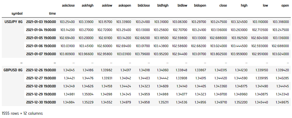
history = qb.history(qb.securities.keys(), datetime(2021, 1, 1), datetime(2021, 12, 31), Resolution.DAILY)
Cointegration
We'll have to test if the assets are cointegrated. If so, we'll have to obtain the cointegration vector(s).
Cointegration Testing
- Select the close column and then call the
unstackmethod. - Call
np.logto convert the close price into log-price series to eliminate compounding effect. - Apply Engle Granger Test to check if the series are cointegrated.
df = history['close'].unstack(level=0)
log_price = np.log(data)
coint_result = engle_granger(log_price.iloc[:, 0], log_price.iloc[:, 1:], trend='n', method='bic')
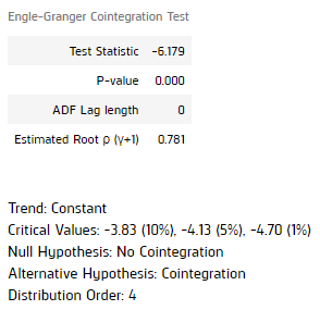
It shows a p-value < 0.05 for the unit test, with lag-level 0. This proven the log price series are cointegrated in realtime. The spread of the 5 forex pairs are stationary.
Get Cointegration Vectors
We would use a VECM model to obtain the cointegrated vectors.
- Initialize a
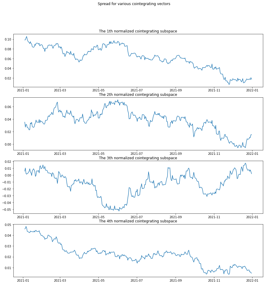
VECMmodel by following the unit test parameters, then fit to our data. - Obtain the
Betaattribute. This is the cointegration subspaces' unit vectors. - Check the spread of different cointegration subspaces.
- Plot the results.
vecm_result = VECM(log_price, k_ar_diff=0, coint_rank=len(assets)-1, deterministic='n').fit()
beta = vecm_result.beta
spread = log_price @ beta
fig, axs = plt.subplots(beta.shape[1], figsize=(15, 15))
fig.suptitle('Spread for various cointegrating vectors')
for i in range(beta.shape[1]):
    axs[i].plot(spread.iloc[:, i])
    axs[i].set_title(f"The {i+1}th normalized cointegrating subspace")
plt.show()
Optimization of Cointegration Subspaces
Although the 4 cointegratoin subspaces are not looking stationarym, we can optimize for a mean-reverting portfolio by putting various weights in different subspaces. We use the Portmanteau statistics as a proxy for the mean reversion. So we formulate:
minimizew(wTM1wwTM0w)2subject towTM0w=ν1Tw=0whereMi≜Cov(st,st+i)=E[(st−E[st])(st+i−E[st+i])T]with s is spread, v is predetermined desirable variance level (the larger the higher the profit, but lower the trading frequency)
- We set the weight on each vector is between -1 and 1. While overall sum is 0.
- Optimize the Portmanteau statistics.
- Normalize the result.
- Plot the weighted spread.
x0 = np.array([-1**i/beta.shape[1] for i in range(beta.shape[1])])
bounds = tuple((-1, 1) for i in range(beta.shape[1]))
constraints = [{'type':'eq', 'fun':lambda x: np.sum(x)}]
opt = minimize(lambda w: ((w.T @ np.cov(spread.T, spread.shift(1).fillna(0).T)[spread.shape[1]:, :spread.shape[1]] @ w)/(w.T @ np.cov(spread.T) @ w))**2,
               x0=x0,
               bounds=bounds,
               constraints=constraints,
               method="SLSQP")
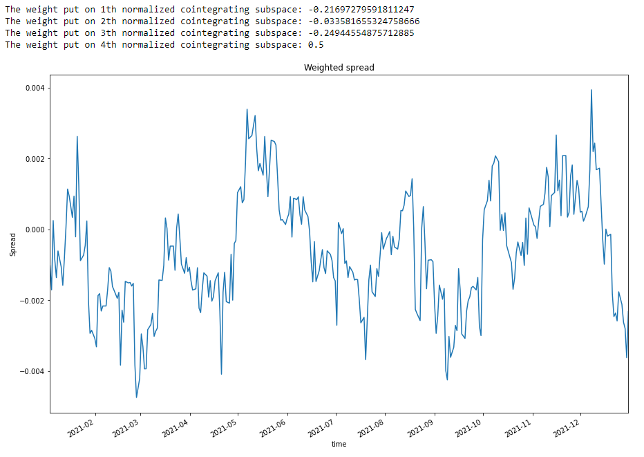
opt.x = opt.x/np.sum(abs(opt.x))
for i in range(len(opt.x)):
    print(f"The weight put on {i+1}th normalized cointegrating subspace: {opt.x[i]}")
new_spread = spread @ opt.x
new_spread.plot(title="Weighted spread", figsize=(15, 10))
plt.ylabel("Spread")
plt.show()
Kalman Filter
The weighted spread looks more stationary. However, the fluctuation half-life is very long accrossing zero. We aim to trade as much as we can to maximize the profit of this strategy. Kalman Filter then comes into the play. It could modify the expectation of the next step based on smoothening the prediction and actual probability distribution of return.
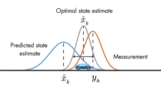
Image Source: Understanding Kalman Filters, Part 3: An Optimal State Estimator. Melda Ulusoy (2017). MathWorks. Retreived from: https://www.mathworks.com/videos/understanding-kalman-filters-part-3-optimal-state-estimator--1490710645421.html
- Initialize a
KalmanFilter. - Obtain the current Mean and Covariance Matrix expectations.
- Initialize a mean series for spread normalization using the
KalmanFilter's results. - Roll over the Kalman Filter to obtain the mean series.
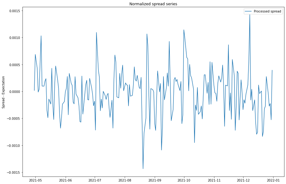
- Obtain the normalized spread series.
- Plot the normalized spread series.
In this example, we use the first 20 data points to optimize its initial state. We assume the market has no regime change so that the transitional matrix and observation matrix is [1].
kalmanFilter = KalmanFilter(transition_matrices = [1],
                  observation_matrices = [1],
                  initial_state_mean = new_spread.iloc[:20].mean(),
                  observation_covariance = new_spread.iloc[:20].var(),
                  em_vars=['transition_covariance', 'initial_state_covariance'])
kalmanFilter = kalmanFilter.em(new_spread.iloc[:20], n_iter=5)
(filtered_state_means, filtered_state_covariances) = kalmanFilter.filter(new_spread.iloc[:20])
currentMean = filtered_state_means[-1, :]
currentCov = filtered_state_covariances[-1, :]
mean_series = np.array([None]*(new_spread.shape[0]-100))
for i in range(100, new_spread.shape[0]):
    (currentMean, currentCov) = kalmanFilter.filter_update(filtered_state_mean = currentMean,
                                                           filtered_state_covariance = currentCov,
                                                           observation = new_spread.iloc[i])
    mean_series[i-100] = float(currentMean)
normalized_spread = (new_spread.iloc[100:] - mean_series)
plt.figure(figsize=(15, 10))
plt.plot(normalized_spread, label="Processed spread")
plt.title("Normalized spread series")
plt.ylabel("Spread - Expectation")
plt.legend()
plt.show()
Determine Trading Threshold
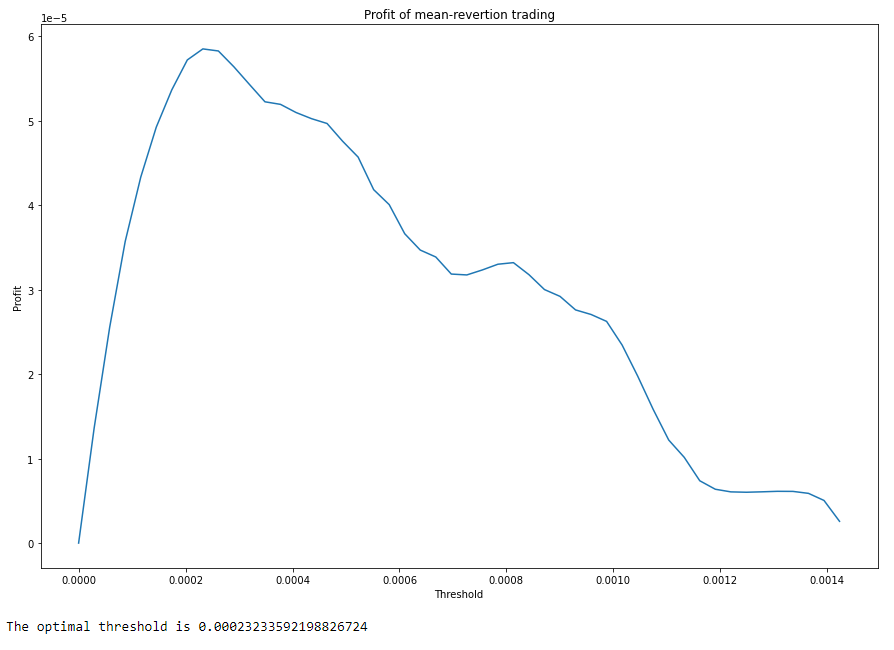
Now we need to determine the threshold of entry. We want to maximize profit from each trade (variance of spread) x frequency of entry. To do so, we formulate:
minimizef‖ˉf−f‖22+λ ‖Df‖22where¯fj=∑Tt=11{spreadt > set levelj}TD=[1−11−1⋱⋱1−1]∈R(j−1)×jso f∗=(I+λDTD)−1ˉf
- Initialize 50 set levels for testing.
- Calculate the profit levels using the 50 set levels.
- Set trading frequency matrix.
- Set level of lambda.
- Obtain the normalized profit level.
- Get the maximum profit level as threshold.
- Plot the result.
s0 = np.linspace(0, max(normalized_spread), 50)
f_bar = np.array([None]*50)
for i in range(50):
    f_bar[i] = len(normalized_spread.values[normalized_spread.values > s0[i]]) / normalized_spread.shape[0]
D = np.zeros((49, 50))
for i in range(D.shape[0]):
    D[i, i] = 1
    D[i, i+1] = -1
l = 1.0
f_star = np.linalg.inv(np.eye(50) + l * D.T@D) @ f_bar.reshape(-1, 1)
s_star = [f_star[i]*s0[i] for i in range(50)]
threshold = s0[s_star.index(max(s_star))]
print(f"The optimal threshold is {threshold}")
plt.figure(figsize=(15, 10))
plt.plot(s0, s_star)
plt.title("Profit of mean-revertion trading")
plt.xlabel("Threshold")
plt.ylabel("Profit")
plt.show()
Test Hypothesis
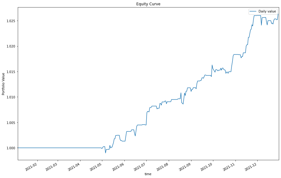
To test the hypothesis. We wish to obtain a profiting strategy.
- Set the trading weight. We would like the portfolio absolute total weight is 1 when trading.
- Set up the trading data.
- Set the buy and sell preiod when the spread exceeds the threshold.
- Trade the portfolio.
- Get the total portfolio value.
- Plot the result.
trading_weight = beta @ opt.x
trading_weight /= np.sum(abs(trading_weight))
testing_ret = data.pct_change().iloc[1:].shift(-1)   # Shift 1 step backward as forward return result
equity = pd.DataFrame(np.ones((testing_ret.shape[0], 1)), index=testing_ret.index, columns=["Daily value"])
buy_period = normalized_spread[normalized_spread < -threshold].index
sell_period = normalized_spread[normalized_spread > threshold].index
equity.loc[buy_period, "Daily value"] = testing_ret.loc[buy_period] @ trading_weight + 1
equity.loc[sell_period, "Daily value"] = testing_ret.loc[sell_period] @ -trading_weight + 1
value = equity.cumprod()
value.plot(title="Equity Curve", figsize=(15, 10))
plt.ylabel("Portfolio Value")
plt.show()
Set Up Algorithm
Once we are confident in our hypothesis, we can export this code into backtesting. One way to accomodate this model into backtest is to create a scheduled event which uses our model to predict the expected return.
def initialize(self) -> None:

    #1. Required: Five years of backtest history
    self.set_start_date(2014, 1, 1)

    #2. Required: Alpha Streams Models:
    self.set_brokerage_model(BrokerageName.ALPHA_STREAMS)

    #3. Required: Significant AUM Capacity
    self.set_cash(1000000)

    #4. Required: Benchmark to SPY
    self.set_benchmark("SPY")

    self.assets = ["EURUSD", "GBPUSD", "USDCAD", "USDHKD", "USDJPY"]

    # Add Equity ------------------------------------------------
    for i in range(len(self.assets)):
        self.add_forex(self.assets[i], Resolution.MINUTE)

    # Instantiate our model
    self.recalibrate()

    # Set a variable to indicate the trading bias of the portfolio
    self.state = 0

    # Set Scheduled Event Method For Recalibrate Our Model Every Week.
    self.schedule.on(self.date_rules.week_start(),
        self.time_rules.at(0, 0),
        self.recalibrate)

    # Set Scheduled Event Method For Kalman Filter updating.
    self.schedule.on(self.date_rules.every_day(),
        self.time_rules.before_market_close("EURUSD"),
        self.every_day_before_market_close)
We'll also need to create a function to train and update our model from time to time. We will switch qb with self and replace methods with their QCAlgorithm counterparts as needed. In this example, this is not an issue because all the methods we used in research also exist in QCAlgorithm.
def recalibrate(self) -> None:
    qb = self
    history = qb.history(self.assets, 252*2, Resolution.DAILY)
    if history.empty:
        return

    # Select the close column and then call the unstack method
    data = history['close'].unstack(level=0)

    # Convert into log-price series to eliminate compounding effect
    log_price = np.log(data)

    ### Get Cointegration Vectors
    # Initialize a VECM model following the unit test parameters, then fit to our data.
    vecm_result = VECM(log_price, k_ar_diff=0, coint_rank=len(self.assets)-1, deterministic='n').fit()

    # Obtain the Beta attribute. This is the cointegration subspaces' unit vectors.
    beta = vecm_result.beta

    # Check the spread of different cointegration subspaces.
    spread = log_price @ beta

    ### Optimization of Cointegration Subspaces
    # We set the weight on each vector is between -1 and 1. While overall sum is 0.
    x0 = np.array([-1**i/beta.shape[1] for i in range(beta.shape[1])])
    bounds = tuple((-1, 1) for i in range(beta.shape[1]))
    constraints = [{'type':'eq', 'fun':lambda x: np.sum(x)}]

    # Optimize the Portmanteau statistics
    opt = minimize(lambda w: ((w.T @ np.cov(spread.T, spread.shift(1).fillna(0).T)[spread.shape[1]:, :spread.shape[1]] @ w)/(w.T @ np.cov(spread.T) @ w))**2,
                    x0=x0,
                    bounds=bounds,
                    constraints=constraints,
                    method="SLSQP")

    # Normalize the result
    opt.x = opt.x/np.sum(abs(opt.x))
    new_spread = spread @ opt.x

    ### Kalman Filter
    # Initialize a Kalman Filter. Using the first 20 data points to optimize its initial state. We assume the market has no regime change so that the transitional matrix and observation matrix is [1].
    self.kalman_filter = kalman_filter(transition_matrices = [1],
                        observation_matrices = [1],
                        initial_state_mean = new_spread.iloc[:20].mean(),
                        observation_covariance = new_spread.iloc[:20].var(),
                        em_vars=['transition_covariance', 'initial_state_covariance'])
    self.kalman_filter = self.kalman_filter.em(new_spread.iloc[:20], n_iter=5)
    (filtered_state_means, filtered_state_covariances) = self.kalman_filter.filter(new_spread.iloc[:20])

    # Obtain the current Mean and Covariance Matrix expectations.
    self.current_mean = filtered_state_means[-1, :]
    self.current_cov = filtered_state_covariances[-1, :]

    # Initialize a mean series for spread normalization using the Kalman Filter's results.
    mean_series = np.array([None]*(new_spread.shape[0]-20))

    # Roll over the Kalman Filter to obtain the mean series.
    for i in range(20, new_spread.shape[0]):
        (self.current_mean, self.current_cov) = self.kalman_filter.filter_update(filtered_state_mean = self.current_mean,
                                                                filtered_state_covariance = self.current_cov,
                                                                observation = new_spread.iloc[i])
        mean_series[i-20] = float(self.current_mean)

    # Obtain the normalized spread series.
    normalized_spread = (new_spread.iloc[20:] - mean_series)

    ### Determine Trading Threshold
    # Initialize 50 set levels for testing.
    s0 = np.linspace(0, max(normalized_spread), 50)

    # Calculate the profit levels using the 50 set levels.
    f_bar = np.array([None]*50)
    for i in range(50):
        f_bar[i] = len(normalized_spread.values[normalized_spread.values > s0[i]]) \
            / normalized_spread.shape[0]

    # Set trading frequency matrix.
    D = np.zeros((49, 50))
    for i in range(D.shape[0]):
        D[i, i] = 1
        D[i, i+1] = -1

    # Set level of lambda.
    l = 1.0

    # Obtain the normalized profit level.
    f_star = np.linalg.inv(np.eye(50) + l * D.T@D) @ f_bar.reshape(-1, 1)
    s_star = [f_star[i]*s0[i] for i in range(50)]
    self.threshold = s0[s_star.index(max(s_star))]

    # Set the trading weight. We would like the portfolio absolute total weight is 1 when trading.
    trading_weight = beta @ opt.x
    self.trading_weight = trading_weight / np.sum(abs(trading_weight))
Now we export our model into the scheduled event method for trading. We will switch qb with self and replace methods with their QCAlgorithm counterparts as needed. In this example, this is not an issue because all the methods we used in research also exist in QCAlgorithm.
def every_day_before_market_close(self) -> None:
    qb = self

    # Get the real-time log close price for all assets and store in a Series
    series = pd.Series()
    for symbol in qb.securities.keys():
        series[symbol] = np.log(qb.securities[symbol].close)

    # Get the spread
    spread = series @ self.trading_weight

    # Update the Kalman Filter with the Series
    (self.current_mean, self.current_cov) = self.kalman_filter.filter_update(filtered_state_mean = self.current_mean,
                                                                        filtered_state_covariance = self.current_cov,
                                                                        observation = spread)

    # Obtain the normalized spread.
    normalized_spread = spread - self.current_mean

    # ==============================

    # Mean-reversion
    if normalized_spread < -self.threshold:
        orders = []
        for i in range(len(self.assets)):
            orders.append(PortfolioTarget(self.assets[i], self.trading_weight[i]))
            self.set_holdings(orders)

        self.state = 1

    elif normalized_spread > self.threshold:
        orders = []
        for i in range(len(self.assets)):
            orders.append(PortfolioTarget(self.assets[i], -1 * self.trading_weight[i]))
            self.set_holdings(orders)

        self.state = -1

    # Out of position if spread recovered
    elif self.state == 1 and normalized_spread > -self.threshold or self.state == -1 and normalized_spread < self.threshold:
        self.liquidate()

        self.state = 0
Examples
The below code snippets concludes the above jupyter research notebook content.
from arch.unitroot.cointegration import engle_granger
from pykalman import KalmanFilter
from scipy.optimize import minimize
from statsmodels.tsa.vector_ar.vecm import VECM

import numpy as np
from matplotlib import pyplot as plt
from pandas.plotting import register_matplotlib_converters
register_matplotlib_converters()

# Instantiate a QuantBook.
qb = QuantBook()

# Select the desired tickers for research.
assets = ["EURUSD", "GBPUSD", "USDCAD", "USDHKD", "USDJPY"]

# Call the AddForex method with the tickers, and its corresponding resolution. Then store their Symbols. Resolution.Minute is used by default.
for i in range(len(assets)):
    qb.add_forex(assets[i],Resolution.MINUTE).symbol

# Call the History method with qb.Securities.Keys for all tickers, time argument(s), and resolution to request historical data for the symbol.
history = qb.history(qb.securities.keys(), datetime(2021, 1, 1), datetime(2021, 12, 31), Resolution.DAILY)

# Select the close column and then call the unstack method.
data = history['close'].unstack(level=0)

# Convert into log-price series to eliminate compounding effect.
log_price = np.log(data)

# Apply Engle Granger Test to check if the series are cointegrated.
coint_result = engle_granger(log_price.iloc[:, 0], log_price.iloc[:, 1:], trend='n', method='bic')

# Initialize a VECM model following the unit test parameters, then fit to our data.
vecm_result = VECM(log_price, k_ar_diff=0, coint_rank=len(assets)-1, deterministic='n').fit()

# Obtain the Beta attribute. This is the cointegration subspaces' unit vectors.
beta = vecm_result.beta

# Check the spread of different cointegration subspaces.
spread = log_price @ beta

# Plot the results.
fig, axs = plt.subplots(beta.shape[1], figsize=(15, 15))
fig.suptitle('Spread for various cointegrating vectors')
for i in range(beta.shape[1]):
    axs[i].plot(spread.iloc[:, i])
    axs[i].set_title(f"The {i+1}th normalized cointegrating subspace")
plt.show()

# We set the weight on each vector is between -1 and 1. While overall sum is 0.
x0 = np.array([-1**i/beta.shape[1] for i in range(beta.shape[1])])
bounds = tuple((-1, 1) for i in range(beta.shape[1]))
constraints = [{'type':'eq', 'fun':lambda x: np.sum(x)}]

# Optimize the Portmanteau statistics.
opt = minimize(lambda w: ((w.T @ np.cov(spread.T, spread.shift(1).fillna(0).T)[spread.shape[1]:, :spread.shape[1]] @ w)/(w.T @ np.cov(spread.T) @ w))**2,
               x0=x0,
               bounds=bounds,
               constraints=constraints,
               method="SLSQP")

# Normalize the result.
opt.x = opt.x/np.sum(abs(opt.x))
for i in range(len(opt.x)):
    print(f"The weight put on {i+1}th normalized cointegrating subspace: {opt.x[i]}")

# Plot the weighted spread.
new_spread = spread @ opt.x
new_spread.plot(title="Weighted spread", figsize=(15, 10))
plt.ylabel("Spread")
plt.show()

# Initialize a Kalman Filter. Using the first 20 data points to optimize its initial state. We assume the market has no regime change so that the transitional matrix and observation matrix is [1].
kalman_filter = KalmanFilter(transition_matrices = [1],
                  observation_matrices = [1],
                  initial_state_mean = new_spread.iloc[:20].mean(),
                  observation_covariance = new_spread.iloc[:20].var(),
                  em_vars=['transition_covariance', 'initial_state_covariance'])
kalman_filter = kalman_filter.em(new_spread.iloc[:20], n_iter=5)
(filtered_state_means, filtered_state_covariances) = kalman_filter.filter(new_spread.iloc[:20])

# Obtain the current Mean and Covariance Matrix expectations.
current_mean = filtered_state_means[-1, :]
current_cov = filtered_state_covariances[-1, :]

# Initialize a mean series for spread normalization using the Kalman Filter's results.
mean_series = np.array([None]*(new_spread.shape[0]-100))

# Roll over the Kalman Filter to obtain the mean series.
for i in range(100, new_spread.shape[0]):
    (current_mean, current_cov) = kalman_filter.filter_update(filtered_state_mean = current_mean,
                                                           filtered_state_covariance = current_cov,
                                                           observation = new_spread.iloc[i])
    mean_series[i-100] = float(current_mean)

# Obtain the normalized spread series.
normalized_spread = (new_spread.iloc[100:] - mean_series)

# Plot the normalized spread series.
plt.figure(figsize=(15, 10))
plt.plot(normalized_spread, label="Processed spread")
plt.title("Normalized spread series")
plt.ylabel("Spread - Expectation")
plt.legend()
plt.show()

# Initialize 50 set levels for testing.
s0 = np.linspace(0, max(normalized_spread), 50)

# Calculate the profit levels using the 50 set levels.
f_bar = np.array([None]*50)
for i in range(50):
    f_bar[i] = len(normalized_spread.values[normalized_spread.values > s0[i]]) \
      / normalized_spread.shape[0]

# Set trading frequency matrix.
D = np.zeros((49, 50))
for i in range(D.shape[0]):
    D[i, i] = 1
    D[i, i+1] = -1

# Set level of lambda.
l = 1.0

# Obtain the normalized profit level.
f_star = np.linalg.inv(np.eye(50) + l * D.T@D) @ f_bar.reshape(-1, 1)
s_star = [f_star[i]*s0[i] for i in range(50)]

# Plot the result.
plt.figure(figsize=(15, 10))
plt.plot(s0, s_star)
plt.title("Profit of mean-revertion trading")
plt.xlabel("Threshold")
plt.ylabel("Profit")
plt.show()

threshold = s0[s_star.index(max(s_star))]
print(f"The optimal threshold is {threshold}")

# Set the trading weight. We would like the portfolio absolute total weight is 1 when trading.
trading_weight = beta @ opt.x
trading_weight /= np.sum(abs(trading_weight))

# Set up the trading data.
testing_ret = data.pct_change().iloc[1:].shift(-1)   # Shift 1 step backward as forward return result
equity = pd.DataFrame(np.ones((testing_ret.shape[0], 1)), index=testing_ret.index, columns=["Daily value"])

# Set the buy and sell preiod when the spread exceeds the threshold.
buy_period = normalized_spread[normalized_spread < -threshold].index
sell_period = normalized_spread[normalized_spread > threshold].index

# Trade the portfolio.
equity.loc[buy_period, "Daily value"] = testing_ret.loc[buy_period] @ trading_weight + 1
equity.loc[sell_period, "Daily value"] = testing_ret.loc[sell_period] @ -trading_weight + 1

# Get the total portfolio value.
value = equity.cumprod()

# Plot the result.
value.plot(title="Equity Curve", figsize=(15, 10))
plt.ylabel("Portfolio Value")
plt.show()
The below code snippets concludes the algorithm set up.
from pykalman import KalmanFilter
from scipy.optimize import minimize
from statsmodels.tsa.vector_ar.vecm import VECM

class KalmanFilterStatisticalArbitrageDemo(QCAlgorithm):

    def initialize(self) -> None:
        #1. Required: Five years of backtest history
        self.set_start_date(2014, 1, 1)
        self.set_end_date(2019, 1, 1)

        #2. Required: Alpha Streams Models:
        self.set_brokerage_model(BrokerageName.ALPHA_STREAMS)

        #3. Required: Significant AUM Capacity
        self.set_cash(1000000)

        #4. Required: Benchmark to SPY
        self.set_benchmark("SPY")

        self.assets = ["EURUSD", "GBPUSD", "USDCAD", "USDHKD", "USDJPY"]

        # Add Equity ------------------------------------------------
        for i in range(len(self.assets)):
            self.add_forex(self.assets[i], Resolution.MINUTE).symbol

        # Instantiate our model
        self.recalibrate()

        # Set a variable to indicate the trading bias of the portfolio
        self.state = 0

        # Set Scheduled Event Method For Kalman Filter updating.
        self.schedule.on(self.date_rules.week_start(),
            self.time_rules.at(0, 0),
            self.recalibrate)

        # Set Scheduled Event Method For Kalman Filter updating.
        self.schedule.on(self.date_rules.every_day(),
            self.time_rules.before_market_close("EURUSD"),
            self.every_day_before_market_close)


    def recalibrate(self) -> None:
        qb = self
        history = qb.history(self.assets, 252*2, Resolution.DAILY)
        if history.empty:
            return

        # Select the close column and then call the unstack method
        data = history['close'].unstack(level=0)

        # Convert into log-price series to eliminate compounding effect
        log_price = np.log(data)

        ### Get Cointegration Vectors
        # Initialize a VECM model following the unit test parameters, then fit to our data.
        vecm_result = VECM(log_price, k_ar_diff=0, coint_rank=len(self.assets)-1, deterministic='n').fit()

        # Obtain the Beta attribute. This is the cointegration subspaces' unit vectors.
        beta = vecm_result.beta

        # Check the spread of different cointegration subspaces.
        spread = log_price @ beta

        ### Optimization of Cointegration Subspaces
        # We set the weight on each vector is between -1 and 1. While overall sum is 0.
        x0 = np.array([-1**i/beta.shape[1] for i in range(beta.shape[1])])
        bounds = tuple((-1, 1) for i in range(beta.shape[1]))
        constraints = [{'type':'eq', 'fun':lambda x: np.sum(x)}]

        # Optimize the Portmanteau statistics
        opt = minimize(lambda w: ((w.T @ np.cov(spread.T, spread.shift(1).fillna(0).T)[spread.shape[1]:, :spread.shape[1]] @ w)/(w.T @ np.cov(spread.T) @ w))**2,
                       x0=x0,
                       bounds=bounds,
                       constraints=constraints,
                       method="SLSQP")

        # Normalize the result
        opt.x = opt.x/np.sum(abs(opt.x))
        new_spread = spread @ opt.x

        ### Kalman Filter
        # Initialize a Kalman Filter. Using the first 20 data points to optimize its initial state. We assume the market has no regime change so that the transitional matrix and observation matrix is [1].
        self.kalman_filter = KalmanFilter(transition_matrices = [1],
                          observation_matrices = [1],
                          initial_state_mean = new_spread.iloc[:20].mean(),
                          observation_covariance = new_spread.iloc[:20].var(),
                          em_vars=['transition_covariance', 'initial_state_covariance'])
        self.kalman_filter = self.kalman_filter.em(new_spread.iloc[:20], n_iter=5)
        (filtered_state_means, filtered_state_covariances) = self.kalman_filter.filter(new_spread.iloc[:20])

        # Obtain the current Mean and Covariance Matrix expectations.
        self.current_mean = filtered_state_means[-1, :]
        self.current_cov = filtered_state_covariances[-1, :]

        # Initialize a mean series for spread normalization using the Kalman Filter's results.
        mean_series = np.array([None]*(new_spread.shape[0]-20))

        # Roll over the Kalman Filter to obtain the mean series.
        for i in range(20, new_spread.shape[0]):
            (self.current_mean, self.current_cov) = self.kalman_filter.filter_update(filtered_state_mean = self.current_mean,
                                                                   filtered_state_covariance = self.current_cov,
                                                                   observation = new_spread.iloc[i])
            mean_series[i-20] = float(self.current_mean)

        # Obtain the normalized spread series.
        normalized_spread = (new_spread.iloc[20:] - mean_series)

        ### Determine Trading Threshold
        # Initialize 50 set levels for testing.
        s0 = np.linspace(0, max(normalized_spread), 50)

        # Calculate the profit levels using the 50 set levels.
        f_bar = np.array([None]*50)
        for i in range(50):
            f_bar[i] = len(normalized_spread.values[normalized_spread.values > s0[i]])               / normalized_spread.shape[0]

        # Set trading frequency matrix.
        D = np.zeros((49, 50))
        for i in range(D.shape[0]):
            D[i, i] = 1
            D[i, i+1] = -1

        # Set level of lambda.
        l = 1.0

        # Obtain the normalized profit level.
        f_star = np.linalg.inv(np.eye(50) + l * D.T@D) @ f_bar.reshape(-1, 1)
        s_star = [f_star[i]*s0[i] for i in range(50)]
        self.threshold = s0[s_star.index(max(s_star))]

        # Set the trading weight. We would like the portfolio absolute total weight is 1 when trading.
        trading_weight = beta @ opt.x
        self.trading_weight = trading_weight / np.sum(abs(trading_weight))


    def every_day_before_market_close(self) -> None:
        qb = self

        # Get the real-time log close price for all assets and store in a Series
        series = pd.Series()
        for symbol in qb.securities.Keys:
            series[symbol] = np.log(qb.securities[symbol].close)

        # Get the spread
        spread = series @ self.trading_weight

        # Update the Kalman Filter with the Series
        (self.current_mean, self.current_cov) = self.kalman_filter.filter_update(filtered_state_mean = self.current_mean,
                                                                           filtered_state_covariance = self.current_cov,
                                                                           observation = spread)

        # Obtain the normalized spread.
        normalized_spread = spread - self.current_mean

        # ==============================

        # Mean-reversion
        if normalized_spread < -self.threshold:
            orders = []
            for i in range(len(self.assets)):
                orders.append(PortfolioTarget(self.assets[i], self.trading_weight[i]))
                self.set_holdings(orders)

            self.state = 1

        elif normalized_spread > self.threshold:
            orders = []
            for i in range(len(self.assets)):
                orders.append(PortfolioTarget(self.assets[i], -1 * self.trading_weight[i]))
                self.set_holdings(orders)

            self.state = -1

        # Out of position if spread recovered
        elif self.state == 1 and normalized_spread > -self.threshold or self.state == -1 and normalized_spread < self.threshold:
            self.liquidate()

            self.state = 0
You can also see our Videos. You can also get in touch with us via Discord.
Did you find this page helpful?