
Indicators
Custom Resolutions
Create Subscriptions
You need to subscribe to some market data in order to calculate indicator values.
qb = QuantBook()
symbol = qb.add_equity("SPY").symbol
Create Indicator Timeseries
You need to subscribe to some market data and create an indicator in order to calculate a timeseries of indicator values.
Follow these steps to create an indicator timeseries:
- Get some historical data.
- Create a data-point indicator.
- Create a
RollingWindowfor each attribute of the indicator to hold their values. - Attach a handler method to the indicator that updates the
RollingWindowobjects. - Create a
TradeBarConsolidatorto consolidate data into the custom resolution. - Attach a handler method to feed data into the consolidator and updates the indicator with the consolidated bars.
- Iterate through the historical market data and update the indicator.
- Populate a
DataFramewith the data in theRollingWindowobjects.
# Request historical trading data with the daily resolution.
history = qb.history[TradeBar](symbol, 70, Resolution.DAILY)
In this example, use a 20-period 2-standard-deviation BollingerBands indicator.
bb = BollingerBands(20, 2)
# Create a window dictionary to store RollingWindow objects.
window = {}
# Store the RollingWindow objects, index by key is the property of the indicator.
window['time'] = RollingWindow[DateTime](50)
window["bollingerbands"] = RollingWindow[float](50)
window["lowerband"] = RollingWindow[float](50)
window["middleband"] = RollingWindow[float](50)
window["upperband"] = RollingWindow[float](50)
window["bandwidth"] = RollingWindow[float](50)
window["percentb"] = RollingWindow[float](50)
window["standarddeviation"] = RollingWindow[float](50)
window["price"] = RollingWindow[float](50)
# Define an update function to add the indicator values to the RollingWindow object.
def update_bollinger_band_window(sender: object, updated: IndicatorDataPoint) -> None:
    indicator = sender
    window['time'].add(updated.end_time)
    window["bollingerbands"].add(updated.value)
    window["lowerband"].add(indicator.lower_band.current.value)
    window["middleband"].add(indicator.middle_band.current.value)
    window["upperband"].add(indicator.upper_band.current.value)
    window["bandwidth"].add(indicator.band_width.current.value)
    window["percentb"].add(indicator.percent_b.current.value)
    window["standarddeviation"].add(indicator.standard_deviation.current.value)
    window["price"].add(indicator.price.current.value)

bb.updated += update_bollinger_band_window
When the indicator receives new data, the preceding handler method adds the new IndicatorDataPoint values into the respective RollingWindow.
consolidator = TradeBarConsolidator(timedelta(days=7))
def on_data_consolidated(sender, consolidated):
    bb.update(consolidated.end_time, consolidated.close)
consolidator.data_consolidated += on_data_consolidated
When the consolidator receives 7 days of data, the handler generates a 7-day TradeBar and update the indicator.
for bar in history:
    consolidator.update(bar)
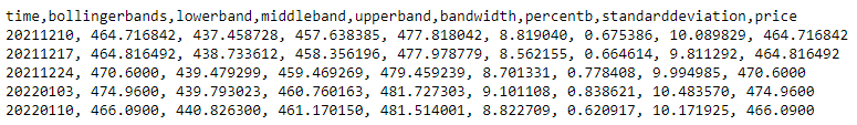
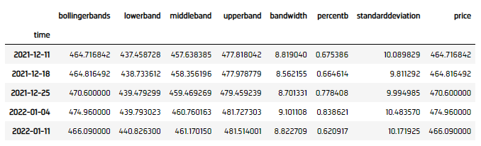
bb_dataframe = pd.DataFrame(window).set_index('time')
Examples
The following examples demonstrate some common practices for researching with data point indicators.
Example 1: Quick Backtest On Bollinger Band
The following example demonstrates a quick backtest to testify the effectiveness of a Bollinger Band mean-reversal, using 5-miunte bar under the research enviornment.
# Instantiate the QuantBook instance for researching.
qb = QuantBook()
# Request SPY data to work with the indicator.
symbol = qb.add_equity("SPY").symbol

# Request historical trading data with the minute resolution.
history = qb.history[TradeBar](symbol, 1000, Resolution.MINUTE)

# Create a window dictionary to store RollingWindow objects.
window = {}
# Store the RollingWindow objects, index by key is the property of the indicator.
window['time'] = RollingWindow[DateTime](50)
window["bollingerbands"] = RollingWindow[float](50)
window["lowerband"] = RollingWindow[float](50)
window["middleband"] = RollingWindow[float](50)
window["upperband"] = RollingWindow[float](50)
window["price"] = RollingWindow[float](50)

# Define an update function to add the indicator values to the RollingWindow object.
def update_bollinger_band_window(sender: object, updated: IndicatorDataPoint) -> None:
    indicator = sender
    window['time'].add(updated.end_time)
    window["bollingerbands"].add(updated.value)
    window["lowerband"].add(indicator.lower_band.current.value)
    window["middleband"].add(indicator.middle_band.current.value)
    window["upperband"].add(indicator.upper_band.current.value)
    window["price"].add(indicator.price.current.value)

# Create the Bollinger Band indicator with parameters to be studied.
bb = BollingerBands(20, 2)
bb.updated += update_bollinger_band_window

# Create a TradeBarConsolidator to consolidate data into the custom resolution.
consolidator = TradeBarConsolidator(timedelta(minutes=5))
# Attach a handler method to feed data into the consolidator and updates the indicator with the consolidated bars.
def on_data_consolidated(sender, consolidated):
    bb.update(consolidated.end_time, consolidated.close)
consolidator.data_consolidated += on_data_consolidated

# Iterate through the historical market data and update the indicator.
for bar in history:
    consolidator.update(bar)

# Populate a DataFrame with the data in the RollingWindow objects.
bb_dataframe = pd.DataFrame(window).set_index('time')

# Create a order record and return column.
# Buy if the asset is underprice (below the lower band), sell if overpriced (above the upper band)
bb_dataframe["position"] = bb_dataframe.apply(lambda x: 1 if x.price < x.lowerband else -1 if x.price > x.upperband else 0, axis=1)
# Get the 1-day forward return.
bb_dataframe["return"] = bb_dataframe["price"].pct_change().shift(-1).fillna(0)
bb_dataframe["return"] = bb_dataframe["position"] * bb_dataframe["return"]

# Obtain the cumulative return curve as a mini-backtest.
equity_curve = (bb_dataframe["return"] + 1).cumprod()
equity_curve.plot(title="Equity Curve on BBand Mean Reversal", ylabel="Equity", xlabel="time")
You can also see our Videos. You can also get in touch with us via Discord.
Did you find this page helpful?