Futures

Follow these steps to subscribe to a Future security:

1. Load the assembly files and data types in their own cell.
C#

#load "../Initialize.csx"

2. Import the data types.
C#

#load "../QuantConnect.csx"
#r "../Microsoft.Data.Analysis.dll"

using QuantConnect;
using QuantConnect.Data;
using QuantConnect.Algorithm;
using QuantConnect.Research;
using QuantConnect.Indicators;
using QuantConnect.Securities.Future;
using Microsoft.Data.Analysis;

3. Create a QuantBook.
Select Language: C#Python

var qb = new QuantBook();

qb = QuantBook()

4. Call the AddFutureadd_future method with a ticker.
Select Language: C#Python

var future = qb.AddFuture(Futures.Indices.SP500EMini);

future = qb.add_future(Futures.Indices.SP_500_E_MINI)

To view the supported assets in the US Futures dataset, see Supported Assets.

5. Set the start date to a date in the past that you want to use as the analysis date.
Select Language: C#Python

qb.SetStartDate(2024, 1, 1);

qb.set_start_date(2024, 1, 1)

The method that you call in the next step returns data on all the contracts that were tradable on this date.

6. Call the FutureChainfuture_chain method with the Symbol of the continuous Futures contract.
Select Language: C#Python

// Get the Futures contracts that were tradable on January 1st, 2024.
var chain = qb.FutureChain(future.Symbol);

# Get the Futures contracts that were tradable on January 1st, 2024.
chain = qb.future_chain(future.symbol, flatten=True)

This method returns a FutureChain object, which represent an entire chain of Futures contracts. You can even format the chain data into a DataFrame where each row in the DataFrame represents a single contract.

7. Sort and filter the data to select the specific contract(s) you want to analyze.
Select Language: C#Python

// Select a contract.
var contractSymbol = chain
    // Select contracts that have at least 1 week before expiry.
    .Where(contract => contract.Expiry > qb.Time.AddDays(7))
    // Select the contract with the largest open interest.
    .OrderByDescending(contract => contract.OpenInterest)
    .First()
    // Get the Symbol of the target contract.
    .Symbol;

# Get the contracts available to trade (in DataFrame format).
chain = chain.data_frame

# Select a contract.
contract_symbol = chain[
    # Select contracts that have at least 1 week before expiry.
    chain.expiry > qb.time + timedelta(7)
    # Select the contract with the largest open interest.
].sort_values('openinterest').index[-1]

8. Call the AddFutureContractadd_future_contract method with a FutureContract Symbol and disable fill-forward.
Select Language: C#Python

qb.AddFutureContract(contractSymbol, fillForward: false);

qb.add_future_contract(contract_symbol, fill_forward=False)

Disable fill-forward because there are only a few OpenInterest data points per day.

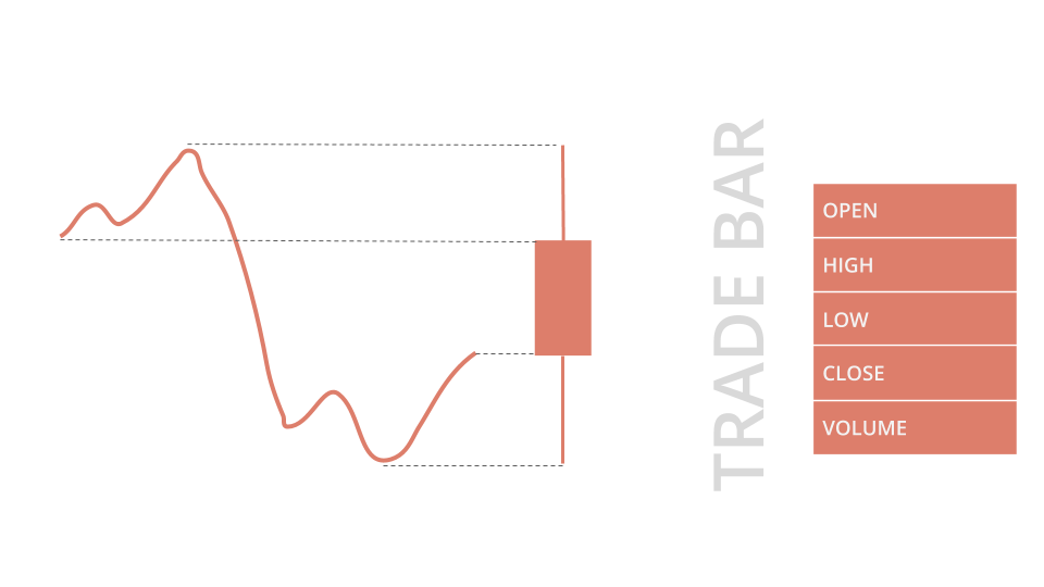
TradeBar objects are price bars that consolidate individual trades from the exchanges. They contain the open, high, low, close, and volume of trading activity over a period of time.

To get trade data, call the history or history[TradeBar]History<TradeBar> method with the contract Symbol object(s).

var history = qb.History<TradeBar>(contractSymbol, TimeSpan.FromDays(3));
foreach (var tradeBar in history)
{
    Console.WriteLine(tradeBar);
}

# DataFrame format
history_df = qb.history(TradeBar, contract_symbol, timedelta(3))
display(history_df)

# TradeBar objects
history = qb.history[TradeBar](contract_symbol, timedelta(3))
for trade_bar in history:
    print(trade_bar)

TradeBar objects have the following properties:

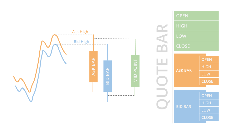
QuoteBar objects are bars that consolidate NBBO quotes from the exchanges. They contain the open, high, low, and close prices of the bid and ask. The Openopen, Highhigh, Lowlow, and Closeclose properties of the QuoteBar object are the mean of the respective bid and ask prices. If the bid or ask portion of the QuoteBar has no data, the Openopen, Highhigh, Lowlow, and Closeclose properties of the QuoteBar copy the values of either the Bidbid or Askask instead of taking their mean.

To get quote data, call the history or history[QuoteBar]History<QuoteBar> method with the contract Symbol object(s).

var history = qb.History<QuoteBar>(contractSymbol, TimeSpan.FromDays(3));
foreach (var quoteBar in history)
{
    Console.WriteLine(quoteBar);
}

# DataFrame format
history_df = qb.history(QuoteBar, contract_symbol, timedelta(3))
display(history_df)

# QuoteBar objects
history = qb.history[QuoteBar](contract_symbol, timedelta(3))
for quote_bar in history:
    print(quote_bar)

QuoteBar objects have the following properties:

To get tick data, call the history or history[Tick]History<Tick> method with the contract Symbol object(s) and Resolution.TICKResolution.Tick.

var history = qb.History<Tick>(contractSymbol, TimeSpan.FromDays(3), Resolution.Tick);
foreach (var tick in history)
{
    Console.WriteLine(tick);
}

# DataFrame format
history_df = qb.history(contract_symbol, timedelta(3), Resolution.TICK)
display(history_df)

# Tick objects
history = qb.history[Tick](contract_symbol, timedelta(3), Resolution.TICK)
for tick in history:
    print(tick)

Tick objects have the following properties:

Tick data is grouped into one millisecond buckets. Ticks are a sparse dataset, so request ticks over a trailing period of time or between start and end times.

Open interest is the number of outstanding contracts that haven't been settled. It provides a measure of investor interest and the market liquidity, so it's a popular metric to use for contract selection. Open interest is calculated once per day.

To get open interest data, call the history or history[OpenInterest]History<OpenInterest> method with the contract Symbol object(s).

var history = qb.History<OpenInterest>(contractSymbol, TimeSpan.FromDays(3));
foreach (var openInterest in history)
{
    Console.WriteLine(openInterest);
}

# DataFrame format
history_df = qb.history(OpenInterest, contract_symbol, timedelta(3))
display(history_df)

# OpenInterest objects
history = qb.history[OpenInterest](contract_symbol, timedelta(3))
for open_interest in history:
    print(open_interest)

OpenInterest objects have the following properties:

The following examples demonstrate some common practices for analyzing Futures data.

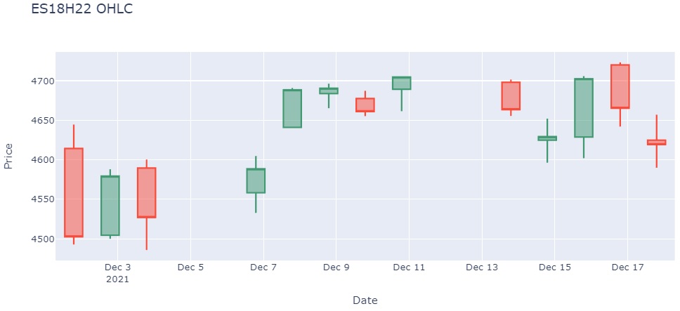
Example 1: Candlestick Chart

The following cells create a candlestick plot for the front-month ES contract:

The following cell creates a candlestick plot for the front-month ES contract:

import plotly.graph_objects as go

qb = QuantBook()
# Get the front-month ES contract as of December 31, 2021.
future = qb.add_future(Futures.Indices.SP_500_E_MINI)
qb.set_start_date(2021, 12, 31)
chain = qb.future_chain(future.symbol)
contract_symbol = list(chain)[0].symbol
# Get the trailing 30 days of trade data for this contract.
history = qb.history(contract_symbol, timedelta(30), Resolution.DAILY).loc[contract_symbol.id.date, contract_symbol]
# Create a candlestick plot with the data.
go.Figure(
    data=go.Candlestick(
        x=history.index,
        open=history['open'],
        high=history['high'],
        low=history['low'],
        close=history['close']
    ), 
    layout=go.Layout(
        title=go.layout.Title(text=f'{contract_symbol.value} OHLC'),
        xaxis_title='Date',
        yaxis_title='Price',
        xaxis_rangeslider_visible=False
    )
).show()

#load "../Initialize.csx"

#r "../Plotly.NET.dll"
using Plotly.NET;
using Plotly.NET.LayoutObjects;

#load "../QuantConnect.csx"
using QuantConnect;
using QuantConnect.Data;
using QuantConnect.Research;
using QuantConnect.Securities;
using QuantConnect.Data.Market;
    
var qb = new QuantBook();
// Get the front-month ES contract as of December 31, 2021.
var future = qb.AddFuture(Futures.Indices.SP500EMini);
qb.SetStartDate(2021, 12, 31);
var contractSymbol = qb.FutureChain(future.Symbol).First().Symbol;
// Get the trailing 30 days of trade data for this contract.
var history = qb.History<TradeBar>(contractSymbol, TimeSpan.FromDays(30), Resolution.Daily);
// Create a candlestick plot with the data.
var chart = Chart2D.Chart.Candlestick<decimal, decimal, decimal, decimal, DateTime, string>(
    history.Select(x => x.Open),
    history.Select(x => x.High),
    history.Select(x => x.Low),
    history.Select(x => x.Close),
    history.Select(x => x.EndTime)
);

LinearAxis xAxis = new LinearAxis();
xAxis.SetValue("title", "Time");
LinearAxis yAxis = new LinearAxis();
yAxis.SetValue("title", "Price ($)");
Title title = Title.init($"{contractSymbol} OHLC");

Layout layout = new Layout();
layout.SetValue("xaxis", xAxis);
layout.SetValue("yaxis", yAxis);
layout.SetValue("title", title);

chart.WithLayout(layout);
HTML(GenericChart.toChartHTML(chart))

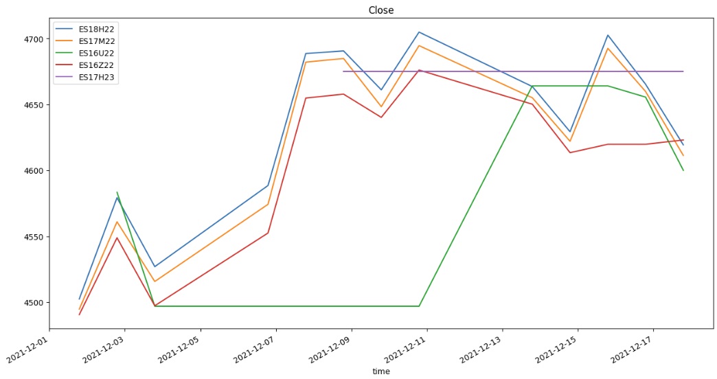
Example 2: Line Chart

The following cells create a line chart for the open interest of the front-month ES contract:

The following cell creates a line plot for all the tradable ES contracts:

import plotly.graph_objects as go

qb = QuantBook()
# Get all the ES contract that were tradable on December 18, 2021.
future = qb.add_future(Futures.Indices.SP_500_E_MINI)
qb.set_start_date(2021, 12, 18)
chain = qb.future_chain(future.symbol)
contract_symbols = [c.symbol for c in chain]
# Get the trailing trade data for these contracts.
history = qb.history(contract_symbols, timedelta(17), Resolution.DAILY)
history.index = history.index.droplevel(0)
closing_prices = history['close'].unstack(level=0)
# Rename the DataFrame columns so the plot legend is readable.
closing_prices.columns = [Symbol.get_alias(x.id) for x in closing_prices.columns]
# Create the line plot.
closing_prices.plot(title="Close", figsize=(15, 8));

#load "../Initialize.csx"

#r "../Plotly.NET.dll"
using Plotly.NET;
using Plotly.NET.LayoutObjects;

#load "../QuantConnect.csx"
using QuantConnect;
using QuantConnect.Data;
using QuantConnect.Research;
using QuantConnect.Securities;
using QuantConnect.Data.Market;
    
var qb = new QuantBook();
// Get the front-month ES contract as of December 31, 2021.
var future = qb.AddFuture(Futures.Indices.SP500EMini);
qb.SetStartDate(2021, 12, 31);
var contractSymbol = qb.FutureChain(future.Symbol).First().Symbol;
// Get the trailing 30 days of open interest data for this contract.
var history = qb.History<OpenInterest>(contractSymbol, TimeSpan.FromDays(30), Resolution.Daily);
// Create a line plot with the data.
var chart = Chart2D.Chart.Line<DateTime, decimal, string>(
    history.Select(x => x.EndTime),
    history.Select(x => x.Value)
);

LinearAxis xAxis = new LinearAxis();
xAxis.SetValue("title", "Time");
LinearAxis yAxis = new LinearAxis();
yAxis.SetValue("title", "Open Interest");
Title title = Title.init($"{contractSymbol} Open Interest");

Layout layout = new Layout();
layout.SetValue("xaxis", xAxis);
layout.SetValue("yaxis", yAxis);
layout.SetValue("title", title);

chart.WithLayout(layout);
HTML(GenericChart.toChartHTML(chart))