Indicators

You need to subscribe to some market data in order to calculate indicator values.

var qb = new QuantBook();
var symbol = qb.AddEquity("SPY").Symbol;

qb = QuantBook()
symbol = qb.add_equity("SPY").symbol

You need to subscribe to some market data and create an indicator in order to calculate a timeseries of indicator values. In this example, use a 20-period 2-standard-deviation BollingerBands indicator.

var bb = new BollingerBands(20, 2);

bb = BollingerBands(20, 2)

You can create the indicator timeseries with the Indicator helper method or you can manually create the timeseries.

Indicator Helper Method

To create an indicator timeseries with the helper method, call the Indicator method.

// Create a dataframe with a date index, and columns are indicator values.
var bbIndicator = qb.Indicator(bb, symbol, 50, Resolution.Daily);

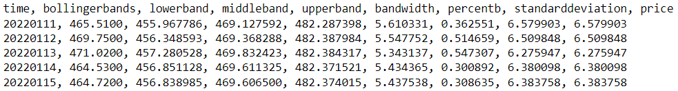
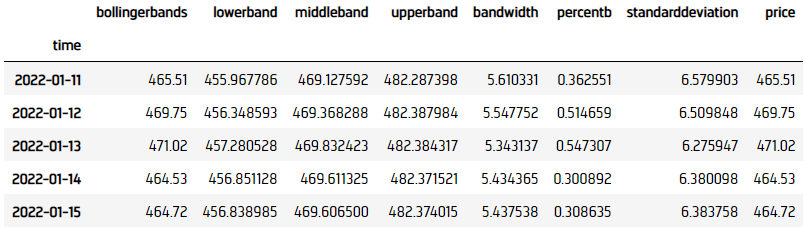
# Create a dataframe with a date index, and columns are indicator values.
bb_dataframe = qb.indicator(bb, symbol, 50, Resolution.DAILY)

Manually Create the Indicator Timeseries

Follow these steps to manually create the indicator timeseries:

1. Get some historical data.

// Request historical trading data with the daily resolution.
var history = qb.History(symbol, 70, Resolution.Daily);

# Request historical trading data with the daily resolution.
history = qb.history[TradeBar](symbol, 70, Resolution.DAILY)

2. Set the indicator Window.Sizewindow.size for each attribute of the indicator to hold their values.

// Set the window.size to the desired timeseries length
bb.Window.Size=50;
bb.LowerBand.Window.Size=50;
bb.MiddleBand.Window.Size=50;
bb.UpperBand.Window.Size=50;
bb.BandWidth.Window.Size=50;
bb.PercentB.Window.Size=50;
bb.StandardDeviation.Window.Size=50;
bb.Price.Window.Size=50;

# Set the window.size to the desired timeseries length
bb.window.size=50
bb.lower_band.window.size=50
bb.middle_band.window.size=50
bb.upper_band.window.size=50
bb.band_width.window.size=50
bb.percent_b.window.size=50
bb.standard_deviation.window.size=50
bb.price.window.size=50

3. Iterate through the historical market data and update the indicator.

foreach (var bar in history)
{
    bb.Update(bar.EndTime, bar.Close);
}

for bar in history:
    bb.update(bar.end_time, bar.close)

4. Display the data.

foreach (var i in Enumerable.Range(0, 5).Reverse())
{
    Console.WriteLine($"{bb[i].EndTime:yyyyMMdd} {bb[i].Value:f4} {bb.LowerBand[i].Value:f4} {bb.MiddleBand[i].Value:f4} {bb.UpperBand[i].Value:f4} {bb.BandWidth[i].Value:f4} {bb.PercentB[i].Value:f4} {bb.StandardDeviation[i].Value:f4} {bb.Price[i].Value:f4}");
}


5. Populate a DataFrame with the data in the Indicator object.

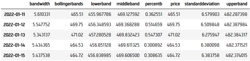
bb_dataframe = pd.DataFrame({
    "current": pd.Series({x.end_time: x.value for x in bb}),
    "lowerband": pd.Series({x.end_time: x.value for x in bb.lower_band}),
    "middleband": pd.Series({x.end_time: x.value for x in bb.middle_band}),
    "upperband": pd.Series({x.end_time: x.value for x in bb.upper_band}),
    "bandwidth": pd.Series({x.end_time: x.value for x in bb.band_width}),
    "percentb": pd.Series({x.end_time: x.value for x in bb.percent_b}),
    "standarddeviation": pd.Series({x.end_time: x.value for x in bb.standard_deviation}),
    "price": pd.Series({x.end_time: x.value for x in bb.price})
}).sort_index()

Jupyter Notebooks don't currently support libraries to plot historical data, but we are working on adding the functionality. Until the functionality is added, use Python to plot data point indicators.

You need to create an indicator timeseries to plot the indicator values.

Follow these steps to plot the indicator values:

1. Select the columns/features to plot.

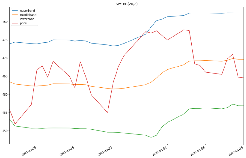
bb_plot = bb_indicator[["upperband", "middleband", "lowerband", "price"]]

2. Call the plot method.

bb_plot.plot(figsize=(15, 10), title="SPY BB(20,2)"))

3. Show the plots.

plt.show()