Research Environment

Universes are data types. To get historical data for a universe, pass the universe data type to the UniverseHistory method. The object that returns contains a universe data collection for each day. With this object, you can iterate through each day and then iterate through the universe data objects of each day to analyze the universe constituents.

For example, follow these steps to get the US Equity Fundamental data for a specific universe:

1. Load the assembly files and data types in their own cell.

#load "../Initialize.csx"

2. Load the necessary assembly files.

#load "../QuantConnect.csx"

3. Import the QuantConnect package and the universe data type.

using QuantConnect;
using QuantConnect.Research;
using QuantConnect.Data.Fundamental;

4. Create a QuantBook.

var qb = new QuantBook();

qb = QuantBook()

5. Define a universe.

The following example defines a dynamic universe that contains the 10 Equities with the lowest PE ratios in the market. To see all the Fundamental attributes you can use to define a filter function for a Fundamental universe, see Data Point Attributes. To create the universe, call the AddUniverseadd_universe method with the filter function.

var universe = qb.AddUniverse(fundamentals =>
{
    return fundamentals
        .Where(f => !double.IsNaN(f.ValuationRatios.PERatio))
        .OrderBy(f => f.ValuationRatios.PERatio)
        .Take(10)
        .Select(f => f.Symbol);
});

def filter_function(fundamentals):
    sorted_by_pe_ratio = sorted(
        [f for f in fundamentals if not np.isnan(f.valuation_ratios.pe_ratio)], 
        key=lambda fundamental: fundamental.valuation_ratios.pe_ratio
    )
    return [fundamental.symbol for fundamental in sorted_by_pe_ratio[:10]]

universe = qb.add_universe(filter_function)

6. Call the UniverseHistoryuniverse_history method with the universe, a start date, and an end date.

var universeHistory = qb.UniverseHistory(universe, new DateTime(2023, 11, 6), new DateTime(2023, 11, 13));

universe_history = qb.universe_history(universe, datetime(2023, 11, 6), datetime(2023, 11, 13))

The end date arguments is optional. If you omit it, the method returns Fundamental data between the start date and the current day.

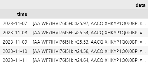
The universe_history method returns a Series where the multi-index is the universe Symbol and the time when universe selection would occur in a backtest. Each row in the data column contains a list of Fundamental objects. The following image shows the first 5 rows of an example Series:



The UniverseHistory method returns an IEnumerable<IEnumerable<Fundamental>> object.

7. Iterate through the Series to access the universe data.
8. Iterate through the result to access the universe data.

universe_history = universe_history.droplevel('symbol', axis=0)
for date, fundamentals in universe_history.items():
    for fundamental in fundamentals:
        symbol = fundamental.symbol
        price = fundamental.price
        if fundamental.has_fundamental_data:
            pe_ratio = fundamental.valuation_ratios.pe_ratio

foreach (var fundamentals in universeHistory)
{
    foreach (Fundamental fundamental in fundamentals)
    {
        var date = fundamental.Time;
        var symbol = fundamental.Symbol;
        var price = fundamental.Price;
        if (fundamental.HasFundamentalData)
        {
            var peRatio = fundamental.ValuationRatios.PERatio;
        }
    }
}

To get universe data for other types of universes, you usually just need to replace Fundamental in the preceding code snippets with the universe data type. The following table shows the datasets that support universe selection and their respective data type. For more information, about universe selection with these datasets and the data points you can use in the filter function, see the dataset's documentation.

To get universe data for Futures and Options, use the FutureHistoryfuture_history and OptionHistoryoption_history methods, respectively.