Popular Libraries

Import the GPlearn library.

from gplearn.genetic import SymbolicRegressor, SymbolicTransformer
from sklearn.model_selection import train_test_split
import joblib

You need the sklearn library to prepare the data and the joblib library to store models.

Get some historical market data to train and test the model. For example, to get data for the SPY ETF during 2020 and 2021, run:

qb = QuantBook()
symbol = qb.add_equity("SPY", Resolution.DAILY).symbol
history = qb.history(symbol, datetime(2020, 1, 1), datetime(2022, 1, 1)).loc[symbol]

You need some historical data to prepare the data for the model. If you have historical data, manipulate it to train and test the model. In this example, use the following features and labels:

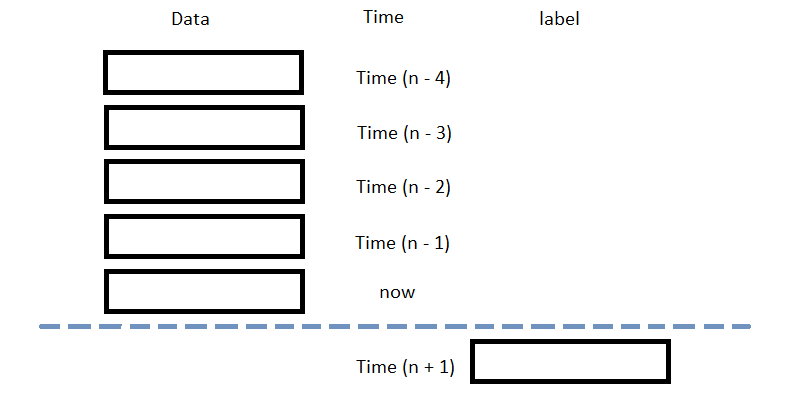
The following image shows the time difference between the features and labels:

Follow these steps to prepare the data:

1. Call the pct_change method and then drop the first row.

daily_returns = history['close'].pct_change()[1:]

2. Loop through the daily_returns DataFrame and collect the features and labels.

n_steps = 5
features = []
labels = []
for i in range(len(daily_returns)-n_steps):
    features.append(daily_returns.iloc[i:i+n_steps].values)
    labels.append(daily_returns.iloc[i+n_steps])

3. Convert the lists of features and labels into numpy arrays.

X = np.array(features)
y = np.array(labels)

4. Split the data into training and testing periods.

X_train, X_test, y_train, y_test = train_test_split(X, y)

You need to prepare the historical data for training before you train the model. If you have prepared the data, build and train the model. In this example, create a Symbolic Transformer to generate new non-linear features and then build a Symbolic Regressor model. Follow these steps to create the model:

1. Declare a set of functions to use for feature engineering.

function_set = ['add', 'sub', 'mul', 'div',
                'sqrt', 'log', 'abs', 'neg', 'inv',
                'max', 'min']

2. Call the SymbolicTransformer constructor with the preceding set of functions.

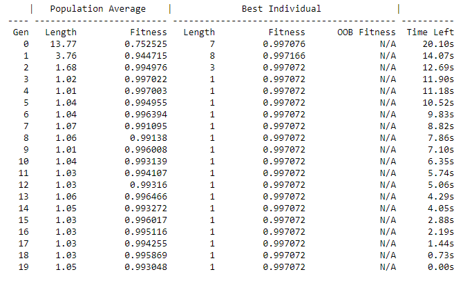
gp_transformer = SymbolicTransformer(function_set=function_set,
                                     random_state=0, 
                                     verbose=1)

3. Call the fit method with the training features and labels.

gp_transformer.fit(X_train, y_train)

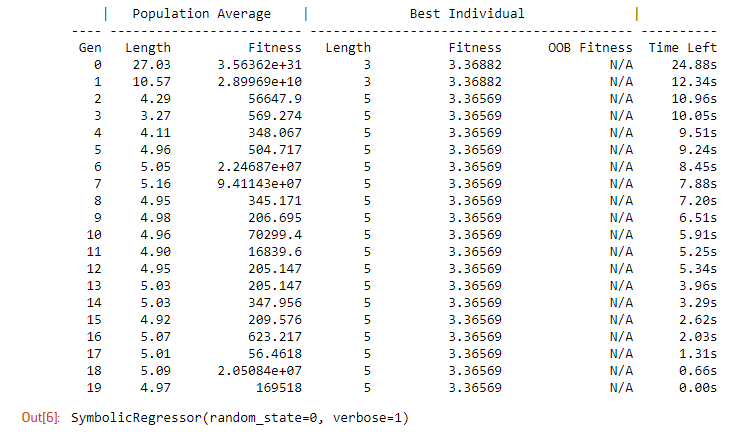
This method displays the following output:


4. Call the transform method with the original features.

gp_features_train = gp_transformer.transform(X_train)

5. Call the hstack method with the original features and the transformed features.

new_X_train = np.hstack((X_train, gp_features_train))

6. Call the SymbolicRegressor constructor.

gp_regressor = SymbolicRegressor(random_state=0, verbose=1)

7. Call the fit method with the engineered features and the original labels.

gp_regressor.fit(new_X_train, y_train)

You need to build and train the model before you test its performance. If you have trained the model, test it on the out-of-sample data. Follow these steps to test the model:

1. Feature engineer the testing set data.

gp_features_test = gp_transformer.transform(X_test)
new_X_test = np.hstack((X_test, gp_features_test))

2. Call the predict method with the engineered testing set data.

y_predict = gp_regressor.predict(new_X_test)

3. Plot the actual and predicted labels of the testing period.

df = pd.DataFrame({'Real': y_test.flatten(), 'Predicted': y_predict.flatten()})
df.plot(title='Model Performance: predicted vs actual closing price', figsize=(15, 10))
plt.show()


4. Calculate the R-square value.

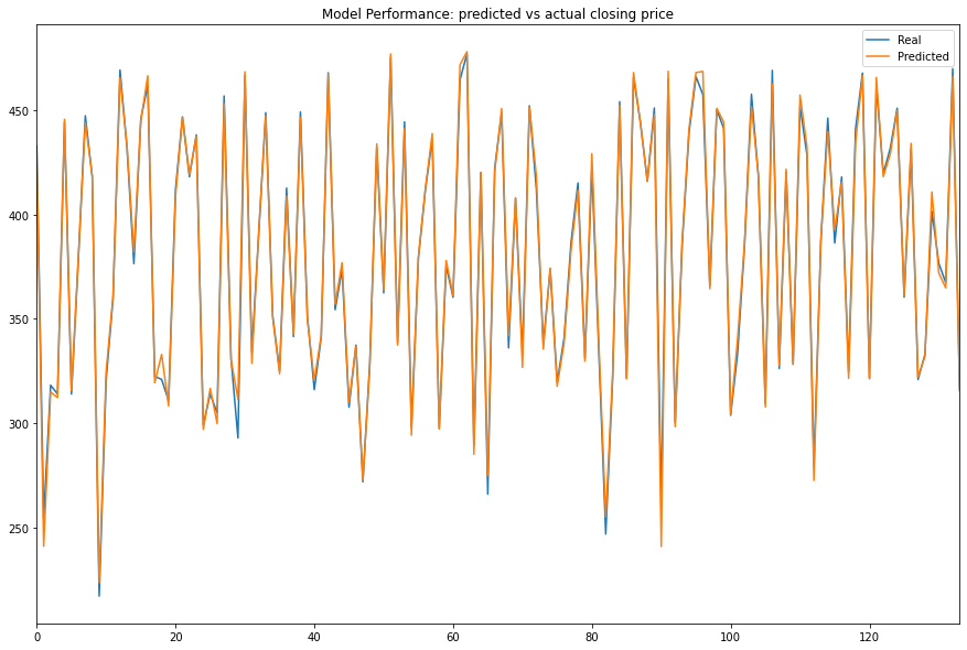
r2 = gp_regressor.score(new_X_test, y_test)
print(f"The explained variance of the GP model: {r2*100:.2f}%")

You can save and load GPlearn models using the Object Store.

Save Models

Follow these steps to save models in the Object Store:

1. Set the key names of the models to be stored in the Object Store.

transformer_key = "transformer"
regressor_key = "regressor"

2. Call the GetFilePathget_file_path method with the key names.

transformer_file = qb.object_store.get_file_path(transformer_key)
regressor_file = qb.object_store.get_file_path(regressor_key)

This method returns the file paths where the models will be stored.

3. Call the dump method with the models and file paths.

joblib.dump(gp_transformer, transformer_file)
joblib.dump(gp_regressor, regressor_file)

If you dump the model using the joblib module before you save the model, you don't need to retrain the model.

Load Models

You must save a model into the Object Store before you can load it from the Object Store. If you saved a model, follow these steps to load it:

1. Call the ContainsKeycontains_key method.

qb.object_store.contains_key(transformer_key)
qb.object_store.contains_key(regressor_key)

This method returns a boolean that represents if the model_key is in the Object Store. If the Object Store does not contain the model_key, save the model using the model_key before you proceed.

2. Call the GetFilePathget_file_path method with the keys.

transformer_file = qb.object_store.get_file_path(transformer_key)
regressor_file = qb.object_store.get_file_path(regressor_key)

This method returns the path where the model is stored.

3. Call the load method with the file paths.

loaded_transformer = joblib.load(transformer_file)
loaded_regressor = joblib.load(regressor_file)

This method returns the saved models.

The following examples demonstrate some common practices for using the GPLearn library.

Example 1: Predict Next Return

The following research notebook uses GPLearn machine learning model to predict the next day's return direction by the previous 5 days' daily returns.

# Import the GPLearn library and others.
from gplearn.genetic import SymbolicRegressor, SymbolicTransformer
from sklearn.model_selection import train_test_split
import joblib

# Instantiate the QuantBook for researching.
qb = QuantBook()
# Request the daily SPY history with the date range to be studied.
symbol = qb.add_equity("SPY", Resolution.DAILY).symbol
history = qb.history(symbol, datetime(2020, 1, 1), datetime(2022, 1, 1)).loc[symbol]

# Obtain the daily returns to be the features and labels.
daily_returns = history['close'].pct_change()[1:]
# We use the previous 5 day returns as the features to be studied.
# Get the 1-day forward return as the labels for the machine to learn.
n_steps = 5
features = []
labels = []
for i in range(len(daily_returns)-n_steps):
    features.append(daily_returns.iloc[i:i+n_steps].values)
    labels.append(daily_returns.iloc[i+n_steps])

# Split the data as a training set and test set for validation.
X = np.array(features)
y = np.array(labels)
X_train, X_test, y_train, y_test = train_test_split(X, y)

# Declare a set of functions to use for feature engineering.
function_set = ['add', 'sub', 'mul', 'div',
                'sqrt', 'log', 'abs', 'neg', 'inv',
                'max', 'min']
# Call the SymbolicTransformer constructor with the preceding set of functions.
gp_transformer = SymbolicTransformer(function_set=function_set,
                                     random_state=0, 
                                     verbose=1)
# Call the fit method with the training features and labels to obtain the set of significant features.
gp_transformer.fit(X_train, y_train)
# Call the transform method to transform the original features.
gp_features_train = gp_transformer.transform(X_train)
# Call the hstack method with the original features and the transformed features to stack them.
new_X_train = np.hstack((X_train, gp_features_train))

# Call the SymbolicRegressor constructor for the non-linear regression fitting.
gp_regressor = SymbolicRegressor(random_state=0, verbose=1)
# Call the fit method with the engineered features and the original labels to fit a non-linear model.
gp_regressor.fit(new_X_train, y_train)

# Feature engineer the testing set data to test with.
gp_features_test = gp_transformer.transform(X_test)
new_X_test = np.hstack((X_test, gp_features_test))
# Call the predict method with the engineered testing set data to get the prediction from the GPLearn model.
y_predict = gp_regressor.predict(new_X_test)

# Plot the actual and predicted labels of the testing period.
df = pd.DataFrame({'Real': y_test.flatten(), 'Predicted': y_predict.flatten()})
df.plot(title='Model Performance: predicted vs actual closing price', figsize=(15, 10))
plt.show()

# Calculate the R-square value to evaluate the model fitness.
r2 = gp_regressor.score(new_X_test, y_test)
print(f"The explained variance of the GP model: {r2*100:.2f}%")

# Predict the label of the testing set data.
y_hat = predict(np.array(X_test))

# Store the model in the object store to allow accessing the model in the next research session or in the algorithm for trading.
transformer_key = "transformer"
regressor_key = "regressor"
transformer_file = qb.object_store.get_file_path(transformer_key)
regressor_file = qb.object_store.get_file_path(regressor_key)
joblib.dump(gp_transformer, transformer_file)
joblib.dump(gp_regressor, regressor_file)