Datasets

You must format the data file into chronological order before you define the custom data class.

To define a custom data class, extend the BaseDataPythonData class and override the GetSource and Reader methods.

#load "../Initialize.csx"
#load "../QuantConnect.csx"
#r "../Microsoft.Data.Analysis.dll"

using QuantConnect;
using QuantConnect.Data;
using QuantConnect.Algorithm;
using QuantConnect.Research;
using Microsoft.Data.Analysis;

public class Nifty : BaseData
{
    public decimal Open;
    public decimal High;
    public decimal Low;
    public decimal Close;

    public Nifty()
    {
    }

    public override SubscriptionDataSource GetSource(SubscriptionDataConfig config, DateTime date, bool isLiveMode)
    {
        var url = "http://cdn.quantconnect.com.s3.us-east-1.amazonaws.com/uploads/CNXNIFTY.csv";
        return new SubscriptionDataSource(url, SubscriptionTransportMedium.RemoteFile);
    }

    public override BaseData Reader(SubscriptionDataConfig config, string line, DateTime date, bool isLiveMode)
    {
        var index = new Nifty();
        index.Symbol = config.Symbol;

        try
        {
            //Example File Format:
            //Date,       Open       High        Low       Close     Volume      Turnover
            //2011-09-13  7792.9    7799.9     7722.65    7748.7    116534670    6107.78
            var data = line.Split(',');
            index.Time = DateTime.Parse(data[0], CultureInfo.InvariantCulture);
            index.EndTime = index.Time.AddDays(1);
            index.Open = Convert.ToDecimal(data[1], CultureInfo.InvariantCulture);
            index.High = Convert.ToDecimal(data[2], CultureInfo.InvariantCulture);
            index.Low = Convert.ToDecimal(data[3], CultureInfo.InvariantCulture);
            index.Close = Convert.ToDecimal(data[4], CultureInfo.InvariantCulture);
            index.Value = index.Close;
        }
        catch
        {
             // Do nothing
        }
        return index;
    }
}

class Nifty(PythonData):
    '''NIFTY Custom Data Class'''
    def get_source(self, config: SubscriptionDataConfig, date: datetime, isLiveMode: bool) -> SubscriptionDataSource:
        url = "http://cdn.quantconnect.com.s3.us-east-1.amazonaws.com/uploads/CNXNIFTY.csv"
        return SubscriptionDataSource(url, SubscriptionTransportMedium.REMOTE_FILE)

    def reader(self, config: SubscriptionDataConfig, line: str, date: datetime, isLiveMode: bool) -> BaseData:
        if not (line.strip() and line[0].isdigit()): return None

        # New Nifty object
        index = Nifty()
        index.symbol = config.symbol

        try:
            # Example File Format:
            # Date,       Open       High        Low       Close     Volume      Turnover
            # 2011-09-13  7792.9    7799.9     7722.65    7748.7    116534670    6107.78
            data = line.split(',')
            index.time = datetime.strptime(data[0], "%Y-%m-%d")
            index.end_time = index.time + timedelta(days=1)
            index.value = data[4]
            index["Open"] = float(data[1])
            index["High"] = float(data[2])
            index["Low"] = float(data[3])
            index["Close"] = float(data[4])

        except:
            pass

        return index

You need to define a custom data class before you can subscribe to it.

Follow these steps to subscribe to custom dataset:

1. Create a QuantBook.

var qb = new QuantBook();

qb = QuantBook()

2. Call the AddData method with a ticker and then save a reference to the data Symbol.

var symbol = qb.AddData<Nifty>("NIFTY").Symbol;

symbol = qb.add_data(Nifty, "NIFTY").symbol

Custom data has its own resolution, so you don't need to specify it.

You need a subscription before you can request historical data for a security. You can request an amount of historical data based on a trailing number of bars, a trailing period of time, or a defined period of time.

Before you request data, call SetStartDate method with a datetimeDateTime to reduce the risk of look-ahead bias.

qb.set_start_date(2014, 7, 29);

qb.set_start_date(2014, 7, 29)

If you call the SetStartDate method, the date that you pass to the method is the latest date for which your history requests will return data.

Trailing Number of Bars

Call the History method with a symbol, integer, and resolution to request historical data based on the given number of trailing bars and resolution.

var history = qb.history(symbol, 10);

history = qb.history(symbol, 10)

This method returns the most recent bars, excluding periods of time when the exchange was closed.

Trailing Period of Time

Call the History method with a symbol, TimeSpantimedelta, and resolution to request historical data based on the given trailing period of time and resolution.

var history = qb.History(symbol, TimeSpan.FromDays(10));

history = qb.history(symbol, timedelta(days=10))

This method returns the most recent bars, excluding periods of time when the exchange was closed.

Defined Period of Time

Call the History method with a symbol, start DateTimedatetime, end DateTimedatetime, and resolution to request historical data based on the defined period of time and resolution. The start and end times you provide are based in the notebook time zone.

var startTime = new DateTime(2013, 7, 29);
var endTime = new DateTime(2014, 7, 29);
var history = qb.History(symbol, startTime, endTime);

start_time = datetime(2013, 7, 29)
end_time = datetime(2014, 7, 29)
history = qb.history(symbol, start_time, end_time)

This method returns the bars that are timestamped within the defined period of time.

In all of the cases above, the History method returns a DataFrame with a MultiIndex.

In all of the cases above, the History method returns an IEnumerable<Nifty> for single-security requests.

Download Method

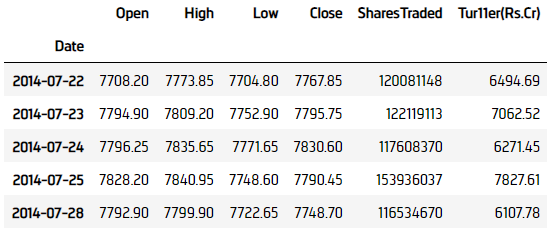
To download the data directly from the remote file location instead of using your custom data class, call the Download method with the data URL.

var content = qb.download("http://cdn.quantconnect.com.s3.us-east-1.amazonaws.com/uploads/CNXNIFTY.csv");

content = qb.download("http://cdn.quantconnect.com.s3.us-east-1.amazonaws.com/uploads/CNXNIFTY.csv")

Follow these steps to convert the content to a DataFrame:

1. Import the StringIO from the io library.

from io import StringIO

2. Create a StringIO.

data = StringIO(content)

3. Call the read_csv method.

dataframe = pd.read_csv(data, index_col=0)

You need some historical data to perform wrangling operations. To display pandas objects, run a cell in a notebook with the pandas object as the last line. To display other data formats, call the print method.

You need some historical data to perform wrangling operations. Use LINQ to wrangle the data and then call the Console.WriteLine method in a Jupyter Notebook to display the data.

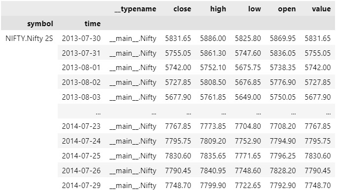
The DataFrame that the History method returns has the following index levels:

1. Dataset Symbol
2. The EndTime of the data sample

The columns of the DataFrame are the data properties.

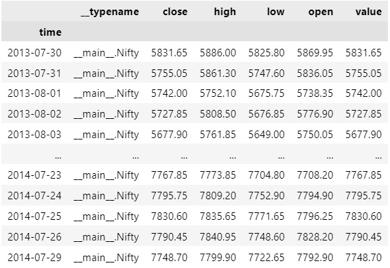
To select the data of a single dataset, index the loc property of the DataFrame with the data Symbol.

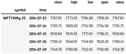
history.loc[symbol]

To select a column of the DataFrame, index it with the column name.

history.loc[symbol]['close']

To get each custom data object, iterate through the result of the history request.

foreach(var nifty in history)
{
    Console.WriteLine($"{nifty} EndTime: {nifty.EndTime}");
}

You need some historical custom data to produce plots. You can use many of the supported plotting librariesPlot.NET package to visualize data in various formats. For example, you can plot candlestick and line charts.

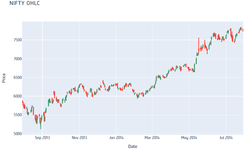
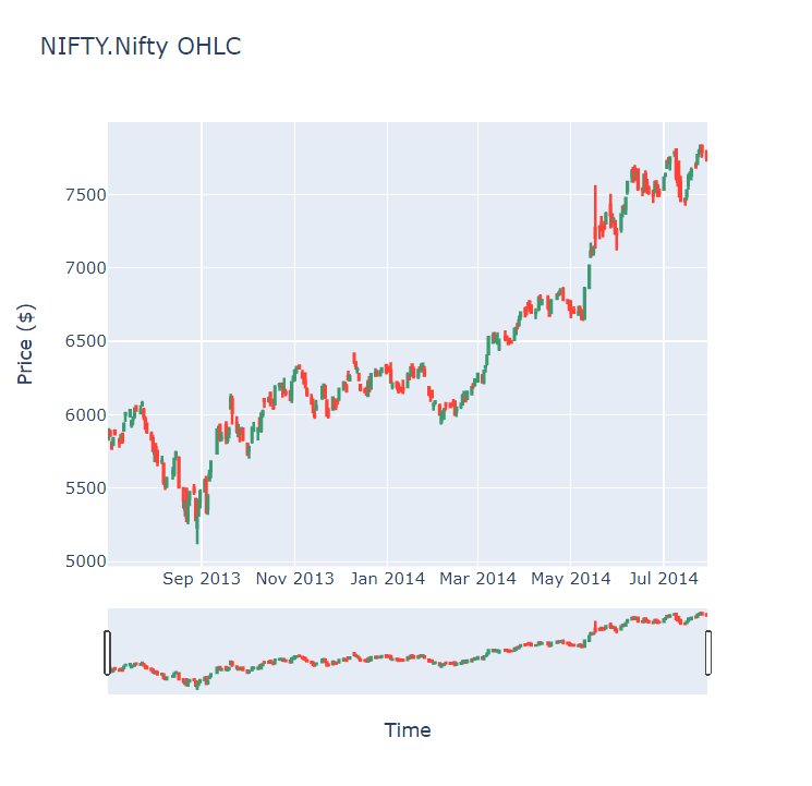
Candlestick Chart

Follow these steps to plot candlestick charts:

1. Get some historical data.

history = qb.history(Nifty, datetime(2013, 7, 1), datetime(2014, 7, 31)).loc[symbol]

var history = qb.History<Nifty>(symbol, new DateTime(2013, 7, 1), new DateTime(2014, 7, 31));

2. Import the plotlyPlot.NET library.

import plotly.graph_objects as go

#r "../Plotly.NET.dll"
using Plotly.NET;
using Plotly.NET.LayoutObjects;

3. Create a Candlestick.
   

candlestick = go.Candlestick(x=history.index,
                             open=history['open'],
                             high=history['high'],
                             low=history['low'],
                             close=history['close'])

var chart = Chart2D.Chart.Candlestick<decimal, decimal, decimal, decimal, DateTime, string>(
    history.Select(x => x.Open),
    history.Select(x => x.High),
    history.Select(x => x.Low),
    history.Select(x => x.Close),
    history.Select(x => x.EndTime)
);

4. Create a Layout.
   

layout = go.Layout(title=go.layout.Title(text=f'{symbol} OHLC'),
                   xaxis_title='Date',
                   yaxis_title='Price',
                   xaxis_rangeslider_visible=False)

LinearAxis xAxis = new LinearAxis();
xAxis.SetValue("title", "Time");
LinearAxis yAxis = new LinearAxis();
yAxis.SetValue("title", "Price ($)");
Title title = Title.init($"{symbol} OHLC");

Layout layout = new Layout();
layout.SetValue("xaxis", xAxis);
layout.SetValue("yaxis", yAxis);
layout.SetValue("title", title);

5. Create a Figure.
   

fig = go.Figure(data=[candlestick], layout=layout)

6. Assign the Layout to the chart.
   

chart.WithLayout(layout);

7. Show the Figure.
   

fig.show()

HTML(GenericChart.toChartHTML(chart))

Candlestick charts display the open, high, low, and close prices of the security.

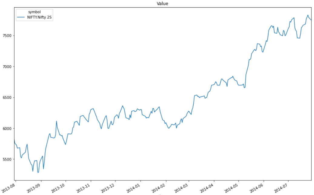
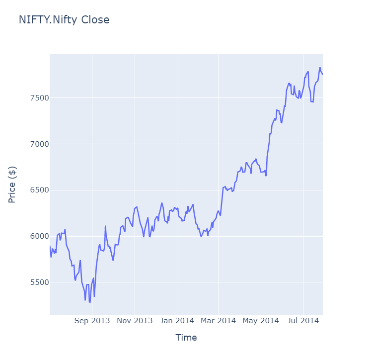
Line Chart

Follow these steps to plot line charts using built-in methodsPlotly.NET package:

1. Select data to plot.

values = history['value'].unstack(level=0)

2. Call the plot method on the pandas object.

values.plot(title="Value", figsize=(15, 10))

3. Create a Line chart.

var chart = Chart2D.Chart.Line<DateTime, decimal, string>(
    history.Select(x => x.EndTime),
    history.Select(x => x.Close)
);

4. Create a Layout.
   

LinearAxis xAxis = new LinearAxis();
xAxis.SetValue("title", "Time");
LinearAxis yAxis = new LinearAxis();
yAxis.SetValue("title", "Price ($)");
Title title = Title.init($"{symbol} Close");

Layout layout = new Layout();
layout.SetValue("xaxis", xAxis);
layout.SetValue("yaxis", yAxis);
layout.SetValue("title", title);

5. Assign the Layout to the chart.
   

chart.WithLayout(layout);

6. Show the plot.

plt.show()

HTML(GenericChart.toChartHTML(chart))

Line charts display the value of the property you selected in a time series.