Research

Indicators allow us to analyze market data in an abstract form rather than in its raw form. For example, indicators like the RSI tell us, based on price and volume data, if the market is overbought or oversold. Because indicators can extract overall market trends from price data, sometimes, we may want to look for correlations between indicators and the market, instead of between raw price data and the market. You can learn more about indicators in the Indicators documentation.

QuantConnect provides over 100+ predefined indicators that you can use in both backtesting and in research. You can find a full list of indicators in the Reference Table. To use an indicator in QuantBook, we will need to define an instance of the indicator object. For example, to define a 10 period Bollinger Band, we will need to provide the period length, the number of standard deviations our bands extend, and the type of moving average.

# Define a 10-period Bollinger bands indicator 
bb = BollingerBands(10, 2, MovingAverageType.Exponential) 

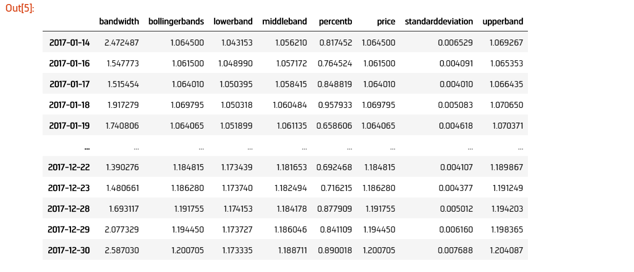
Similar to backtesting, once we have our indicator object, we will need to warm it up with historical data. We can accomplish this using the qb.Indicator helper method, which detects the indicator and data required, and pipes historical data through it. The qb.Indicator method returns a dataframe containing values for our indicator. Each column of the dataframe corresponds to a component of our indicator. For example, for BollingerBands, there is a column for each band.

We can use qb.Indicator(Indicator, Symbol, StartDate, EndDate, Resolution) to warm up an indicator with historical data between two dates.

start_date = datetime(2017,1,1)
end_date = datetime(2018,1,1)

# Generate the indicator value of EURUSD from 2017 to 2018
df1_bb = qb.Indicator(bb, "EURUSD", start_date, end_date, Resolution.Daily)

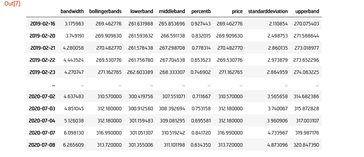
We can also use qb.Indicator(Indicator, Symbol, Period, Resolution) to warm up an indicator with historical data from the last N periods.

# Generate the indicator value of SPY for the last 360 days
df2_bb = qb.Indicator(bb, "SPY", 360, Resolution.Daily) 

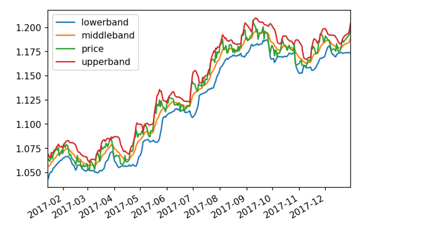
When we use qb.Indicator to warm up an indicator, the indicator values are returned in a pandas dataframe. Because pandas dataframes allow plotting with the df.plot() method, it is straightforward to make simple plots of our indicators;

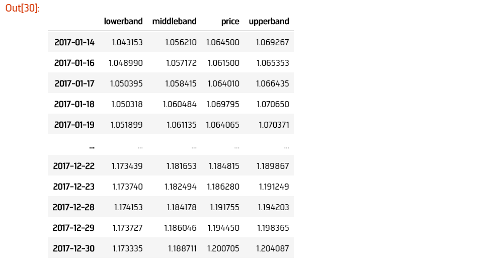
Before we plot our indicator, we should filter out columns in the dataframe which are not relevant to our analysis. For our Bollinger Band indicator, we find that the standard deviation column contains much smaller values than the other columns. This may skew our charts when it scales to fit all the data. We can drop all the irrelevant columns, such as the standarddeviation and percentb columns, from our dataframe before we plot it.

# drop all irrelevant columns fields
df1_bb.drop(['standarddeviation', 'bandwidth', 'percentb', 'bollingerbands'], axis=1, inplace=True)

# plot the Bollinger Band
df1_bb.plot()

Data from history calls is restricted to the default resolutions available for the given type of security, such as second, minute, hour, and daily resolutions. This means that when using qb.Indicator, the resolution of our indicators is also restricted to the default resolutions. If we want to create, for example, a 5-minute resolution indicator, we will need to consolidate our minute resolution historical data into 5 minute data. You can learn how to consolidate data in a pandas dataframe in the Consolidating Historical Data documentation. After consolidating our data, we will need to manually update our indicator with data from our consolidated dataframe and save those indicator values in a new dataframe.

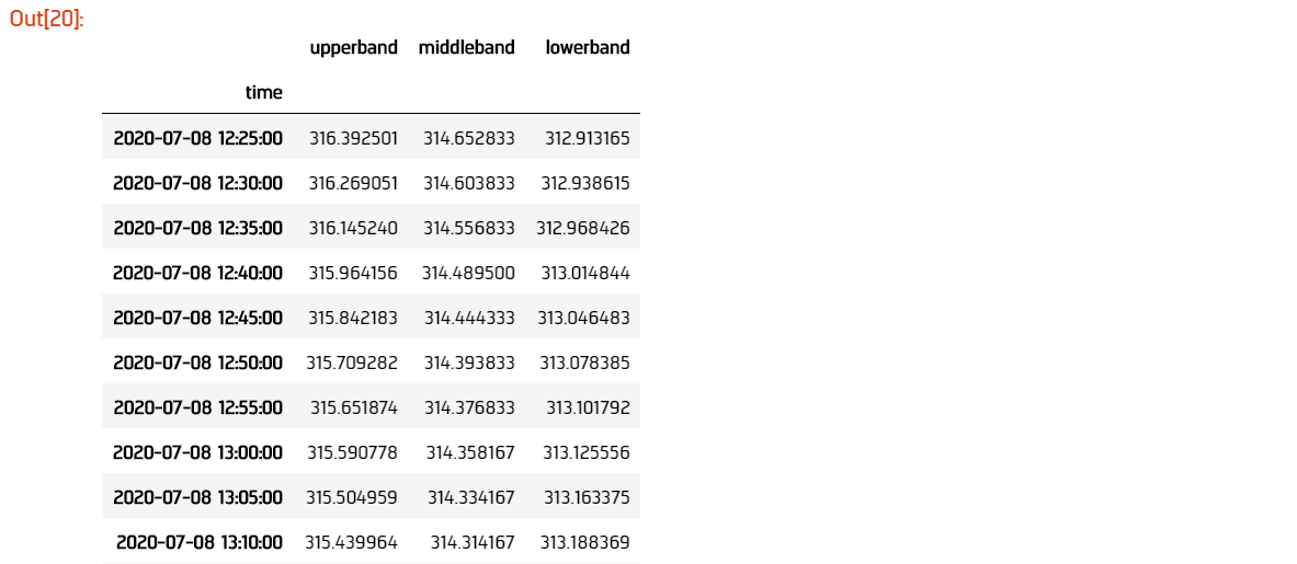
For example, consider the case where we've consolidated our minute historical data into 5 minute data. Let's create a 5 minute Bollinger Band indicator from our new 5 minute dataframe.

# Our consolidated dataframe
df_5min_ohlc

# Our BB indicator
bb = BollingerBands(30, 2)

# Dictionary to hold consolidated BB values
bb_values = {'time': [], 'upperband': [], 'middleband': [], 'lowerband': []}

# Iterate through consolidated dataframe
for row in df_5min_ohlc.itertuples():
    time = row.Index 
    close = row.close

    # Update indicator with consolidated data
    bb.Update(time, close)

    # If BB values are ready, append data
    if bb.IsReady:
        bb_values['time'].append(time)  # Save timestamps to create index for dataframe
        bb_values['upperband'].append(bb.UpperBand.Current.Value)
        bb_values['middleband'].append(bb.MiddleBand.Current.Value)
        bb_values['lowerband'].append(bb.LowerBand.Current.Value)

# Create indicator dataframe from 
consolidated_bbdf =  pd.DataFrame(bb_values, columns=['time', 'upperband', 'middleband', 'lowerband'])  
# Set index to time
consolidated_bbdf = consolidated_bb.set_index('time') 

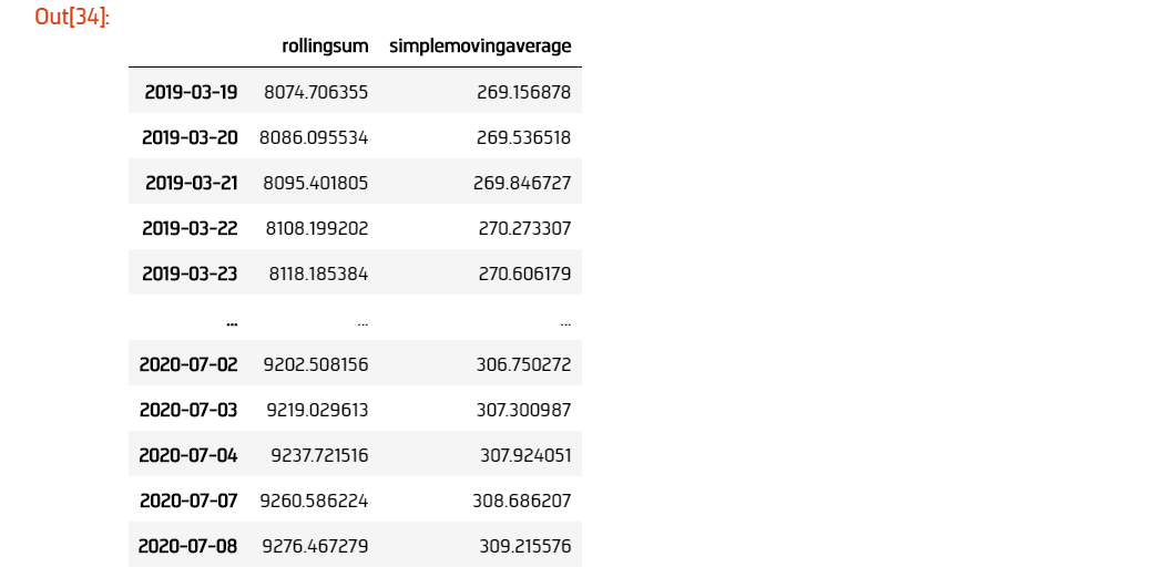
Indicators in Lean can be chained together to create unique combinations corresponding to new indicators. For example, we can compose the SimpleMovingAverage indicator with a RelativeStrengthIndex indicator to create a new indicator which is the SMA of the RSI. This is accomplished by using Indicator Extensions, which let us compose and operate on indicators. You can find a complete list of available Indicator Extensions in the Indicator documentation.

# Create a 14 period RSI indicator
rsi = RelativeStrengthIndex(14)

# Create a 30 period SMA indicator
sma = SimpleMovingAverage(30)

# Compose indicators
sma_of_rsi = IndicatorExtensions.Of(sma, rsi)

df_sma_of_rsi = qb.Indicator(rsiAverage, spy.Symbol, 360, Resolution.Daily)