Research

The Research environment allows you to directly access historical data from any period. This includes Equities, Options, Forex, and Futures data going back as far as 1998. Similar to backtesting, the data is accessed by first subscribing to a security, qb.AddEquity("SPY"), and then making a history call, qb.History("SPY", 10, Resolution.Daily).

The data from the history call is returned in a pandas dataframe. Pandas is a python data manipulation and analysis framework. A pandas dataframe is a 2 dimensional labeled data structure, much like a spreadsheet or SQL table. A label on a row is called an Index and labels on columns are simply called columns.

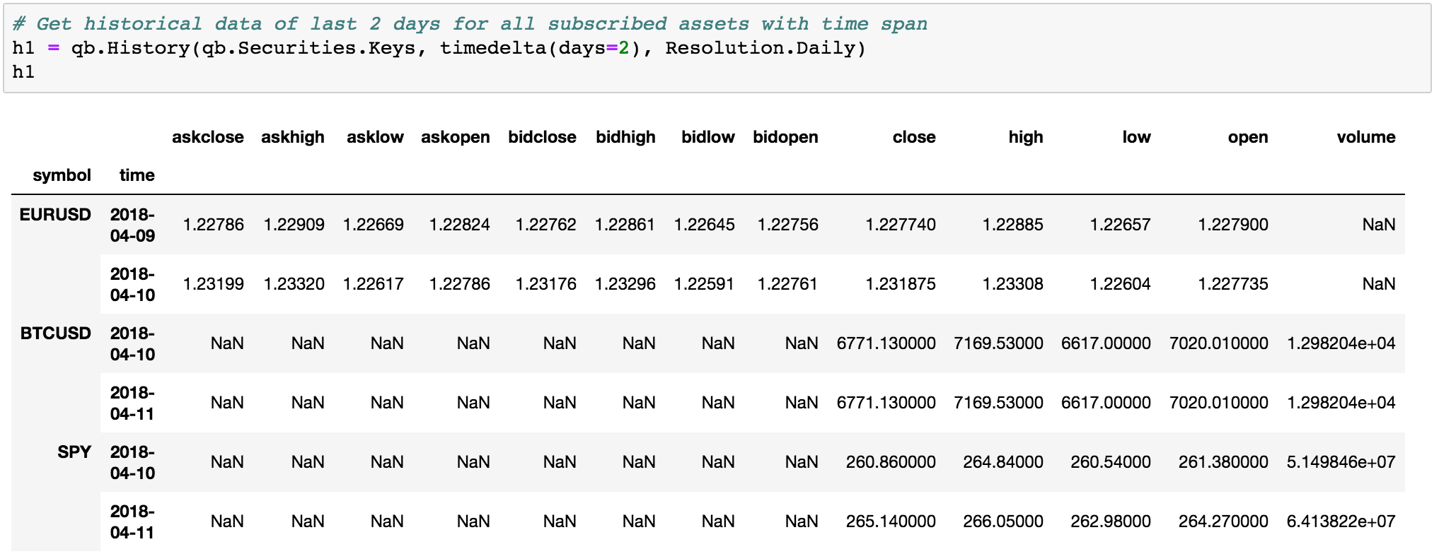
In the example below, a history request is made for all securities that been subscribed to. The resulting data frame has columns for each data type returned; these data types correspond to components of the Trade data or the Quote data available. Notice that because SPY and BTCUSD do not have Quote data, they have NaN values for those columns.

QuantConnect provides Equity data from QuantQuote for over 8000 equities going back as far as 1998. The data is available in tick, second, minute, hour, and daily resolutions. By default, the data is adjusted for dividends and splits. To access the data for a given equity, we must first subscribe to its data using its ticker.

qb = QuantBook()
spy = qb.AddEquity("SPY") # add equity data

Making History Calls

The history call requires you to pass in the symbols you wish to retrieve data for and, the period and resolution of the data. There are three different ways to make a history call:

# Returns the past 10 days of historical daily data
history = qb.History(spy.Symbol, timedelta(days=10), Resolution.Daily)

# Returns the past 10 bars of historical daily data
history = qb.History(spy.Symbol, 10, Resolution.Daily)

start_time = datetime(2019, 1, 1) # start datetime for history call
end_time = datetime(2020, 1, 1) # end datetime for history call

# Returns daily historical data between January 1st 2019 and January 1st 2020
history = qb.History(spy.Symbol, start_time, end_time, Resolution.Daily)

If we have subscribed to multiple symbols, we can retrieve a single dataframe which contains historical data for all our symbols, by using qb.History(qb.Securities.Keys, 10, Resolution.Daily).

spy = qb.AddEquity("SPY")
tlt = qb.AddEquity("TLT")
gld = qb.AddEquity("GLD")

# Returns daily historical data for all symbols
history = qb.History(qb.Securities.Keys, timedelta(days=10), Resolution.Daily)

Accessing and Manipulating Data

The dataframe returned will have a column for each data type available. For equities, the dataframe will have a column for Open, High, Low, Close, and Volume data since equity quote data is not yet available. The rows are indexed by time, meaning each OHLC row correlates to one timestamp. The frequency between timestamps will depend on the resolution of data. Rows are also indexed by symbols if multiple symbols were passed into the history call.

We can use history.loc["SPY"] to access the time series row data for a specific symbol. The row data will contain the open, high, low, close, and volume data for a given timestamp.

history.loc["SPY"]

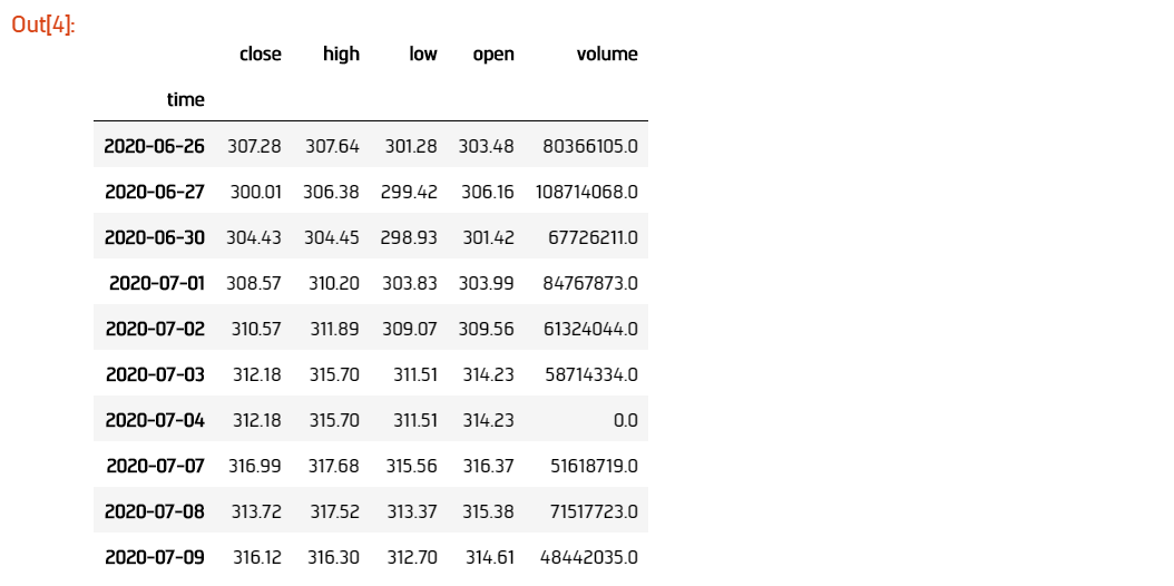
From here, we can then access specific columns. Let's access the time series close data.

history.loc["SPY"]["close"]

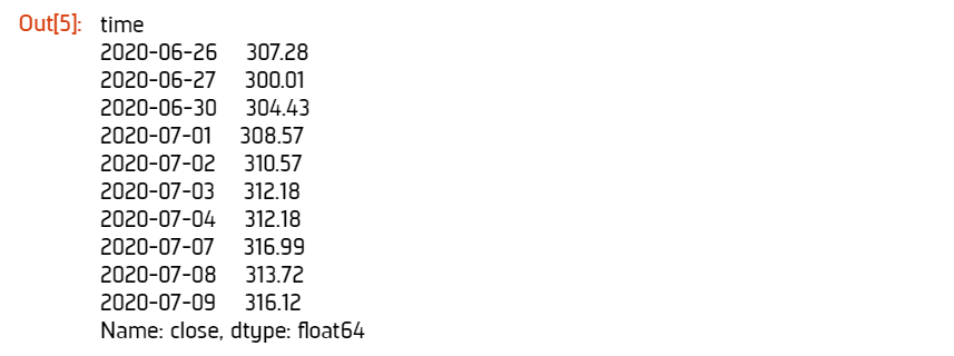
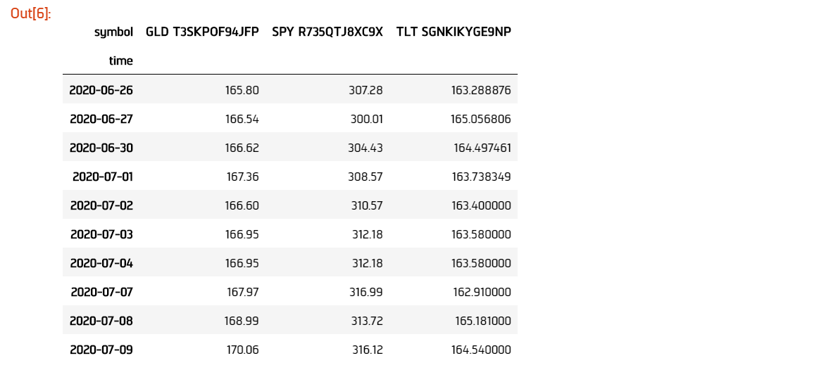
We can also access the time series close data for all symbols by unstacking the dataframe.

history['close'].unstack(level=0)

QuantConnect provides Forex data from both FXCM and Oanda for 71 currency pairs going back as far as 2004. You can find a full list of supported pairs in the data library. The data is available in Tick, Second, Minute, Hour, and Daily resolutions. Unlike equities, Forex data also contains quote data. To access the data for a given pair, we must first subscribe to its data using its ticker.

Making History Calls

qb = QuantBook()
eurusd = qb.AddForex("EURUSD") # add EURUSD data

The history call requires you to pass in the symbols you wish to retrieve data for and, the period and resolution of the data. There are three different ways to make a history call:

# Returns the past 10 days of historical daily data
history = qb.History(eurusd.Symbol, timedelta(days=10), Resolution.Daily)

# Returns the past 10 bars of historical daily data
history = qb.History(eurusd.Symbol, 10, Resolution.Daily)

start_time = datetime(2019, 1, 1) # start datetime for history call
end_time = datetime(2020, 1, 1) # end datetime for history call

# Returns daily historical data between January 1st 2019 and January 1st 2020
history = qb.History(eurusd.Symbol, start_time, end_time, Resolution.Daily)

If we have subscribed to multiple symbols, we can retrieve a single dataframe which contains historical data for all our symbols, by using qb.History(qb.Securities.Keys, 10, Resolution.Daily).

eurusd = qb.AddForex("EURUSD")
gbpusd = qb.AddForex("GBPUSD")
usdjpy = qb.AddForex("USDJPY")

# Returns daily historical data for all symbols
history = qb.History(qb.Securities.Keys, timedelta(days=10), Resolution.Daily)

Accessing and Manipulating Data

The dataframe returned will have a column for each data type available. Similar to equities, the dataframe will have a column for Open, High, Low, Close, and Volume (OHLC) data, but there will also be columns for Ask OHLC and Bid OHLC data. The rows are indexed by time, meaning each row correlates to one timestamp. Rows are also indexed by symbols if multiple symbols were passed into the history call.

We can use history.loc["EURUSD"] to access the time series row data for a specific symbol. The row data will contain the open, high, low, close, volume (OHLC) data and the quote data, which includes Ask OHLC and Bid OHLC data. Each row is indexed by a given timestamp.

history.loc["EURUSD"]

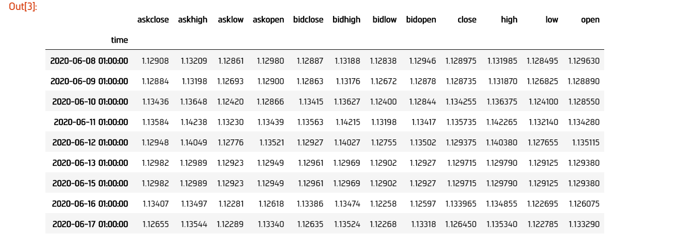
From here, we can then access specific columns. Let's access the time series high data for the ask quote bar.

history.loc["EURUSD"]["askhigh"]

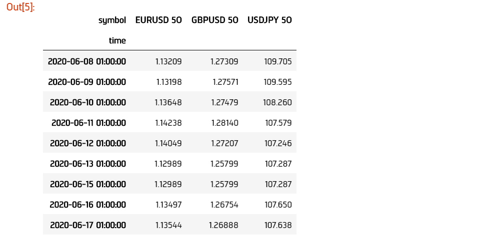
We can also access the time series ask high data for all symbols by unstacking the dataframe.

history['askhigh'].unstack(level=0)

,QuantConnect provides equity options data from AlgoSeek going back as far as 2010. The options data is available only in minute resolution, which means we need to consolidate the data if we wish to work with other resolutions. Options data also contains both trade data and quote data. To access options data, we need to first subscribe to an underlying and also to the option chains data for that underlying.

qb = QuantBook()
spy = qb.AddEquity("SPY") # add SPY data
spy_option = qb.AddOption("SPY") # add SPY option data

Setting a Filter

When we use qb.AddOption("SPY"), we are subscribed to the option chain data for SPY, which contains a large number of contracts with different rights, strikes, and expirations. We need to filter the contracts in the chain for the ones which interest us. We can do this using the Option.SetFilter method. There are a few different ways we can filter our options chain.

One way to refer to a strike price is to use the number of strike levels it is below or above the current market price. If SPY is trading at $300 and the option chain contains strikes: $285, $295, $300, $305, $310, $315, then we can refer to the $290 strike as -2 because it is 2 strikes below the current market price of SPY.

We can filter the chain by the range of strike prices we are interested in. For example, we can restrict the chain to only include contracts with strike prices between -2 strikes and +5 strikes.

spy_option.SetFilter(-2, +5)

We can also filter by the range of expirations for our contracts. For example, let's restrict our chain to contracts expiring between 7 days from now and 30 days from now.

spy_option.SetFilter(timedelta(days=7), timedelta(days=30))

We can combine strike filtering and expiration filtering to narrow our chain even further. We can choose contracts which are expiring between 7 days from now and 30 days from now, whose strikes are also between -2 strikes and +5 strikes.

spy_option.SetFilter(-2, +5, timedelta(days=7), timedelta(days=30))

Making History Calls

Regular qb.History calls do not work for options. Instead, we need to use qb.GetOptionHistory, which allows us to request options data during a given period. 

start_time =  datetime(2017, 1, 11, 10, 10) 
end_time = datetime(2017, 1, 13, 12, 10)

# Request SPY options history between given dates
option_history = qb.GetOptionHistory(spy.Symbol, start_time, end_time)

qb.GetOptionHistory does not return a dataframe of historical data. It instead returns an OptionHistory object, which allows us to access the strike, expiration, and price data.

We can use OptionHistory.GetAllData() to return a dataframe containing all the price data for the options chain. This dataframe contains all the quote, trade and open interest data for each contract in our history call. It is indexed by contract expiry, strike, option right type, contract symbol, and data timestamp.

# Fetch historical price data for options chain
history = option_history.GetAllData()

We can retrieve the set of strike prices for the contracts in our history call.

# Fetch strikes of all options contracts 
option_history.GetStrikes()

We can also access the set of expiries for the contracts in our history call.

# Fetch expiration dates of all options contracts
option_history.GetExpiryDates()

QuantConnect provides trade and quote data from AlgoSeek for over 100 Futures symbols going back as far as 2009. You can find a full list of available Futures symbols in the data library . Futures data is available in tick, second and minute resolutions. To access data for a given Future, we need to first subscribe to its data using its ticker.

# Subcribes to data for S&P500 E-mini Futures (ES).
es = qb.AddFuture("ES")

We can also refer to Future tickers using a predefined categorized Enum. For example, The ticker for S&P 500 E-mini futures ("ES"), can be accessed with Futures.Indices.SP500EMini. This means we can subscribe to data for ES using qb.AddFuture(Futures.Indices.SP500EMini). You can find a full list of all the tickers and their associated Enum addresses in the data library.

Setting a Filter

Futures data for a given commodity contains a chain of contracts of different expirations. We can filter the chain by expiration to narrow the data to contracts which interest us.

# Filter for contracts which are expiring in less than 180 days.
es.SetFilter(timedelta(0), timedelta(180))

Making History Calls

Similar to options, future historical data can't be accessed using qb.History. Instead, we need to use qb.GetFutureHistory, which lets us access historical futures data.

start_time = datetime(2019, 2, 12, 10, 30) # February 12th 2019 10:30 AM
end_time = datetime(2019, 2, 16, 16, 0) # February 16th 2019 4:00 PM

future_history = qb.GetFutureHistory(es.Symbol, start_time, end_time)

qb.GetFutureHistory does not return a dataframe of historical data. It instead returns a FutureHistory object, which lets us access the expiry and price data for the chain.

We can access historical price data using FutureHistory.GetAllData. This returns a dataframe containing quote, trade, and open interest data for the contracts in the future chain. The data is indexed by contract expiry, symbol and the timestamp of the data.

# Get all futures data as a dataframe
history = future_history.GetAllData()

We can also retrieve the list of expiry dates of the futures contracts in our historical call.

# Fetch expiration dates of all futures contracts
future_history.GetExpiryDates()

Raw data from history calls are usually limited to a few different resolutions. If we want to analyze our bar data on custom time frames, such as 5 minute bars or 4 hour bars, we will need to consolidate the raw data.

Resample

One way to consolidate data from our history call is to manipulate our dataframe using the pandas resample method. Resample allows us to convert the frequency of a timeseries dataframe into a custom frequency. Consider an example where we've made a history call for minute resolution data and we want to create 5 minute resolution data.

qb = QuantBook()

spy = qb.AddEquity("SPY")

startDate = datetime(2018, 4, 1)
endDate = datetime(2018, 7, 15)

df = qb.History(spy.Symbol, startDate, endDate, Resolution.Minute)

Note, that the resample method works only on dataframes with a datetime index. The dataframe returned from the history call is a multi-index dataframe, with 2 indices: a symbol index for each security in the dataframe and a time index for the timestamps for each row of data. We need to drop the symbol index from our dataframe so that it is compatible with resample. This is accomplished with the pandas reset_index method.

# Drop level 0 index (symbol index) from dataframe
df.reset_index(level = 0, drop = True, inplace=True)

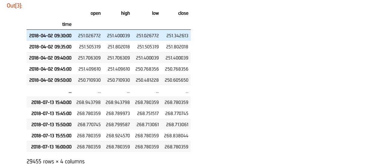
When we use resample, a Resampler object is returned which then needs to be downsampled using one of the pandas downsampling computations. For our purposes, we can use the Resampler.ohlc downsampling method to aggregate our price data.

When we resample our dataframe, an OHLC row will be created for each column in our dataframe. We can simplify our data by looking at the OHLC of just the close column by resampling only the close column. A resample offset of 5T corresponds to a 5 minute resample. Other resampling offsets include: 2D = 2 days; 5H = 5 hours; 3S = 3 seconds.

close_prices = df["close"]

offset = "5T" 
close_5min_ohlc = close_prices.resample(offset).ohlc()