


Abstract
In this tutorial we implement a high frequency and dynamic pairs trading strategy based on market-neutral statistical arbitrage strategy using a two-stage correlation and cointegration approach. This strategy is based on George J. Miao's work. We applied this trading strategy to the U.S. bank sector stocks, backtested this strategy with 10-minute stock data in September 2013. Our trading strategy yields a compounding annual return up to 26.924% and a 3.011 Sharpe ratio.
This strategy is especially profitable when the market is performing poorly. The profit is resulted from mispricing, and mispricings are likely to happen when the market goes down or volatility increases.
This example is a basic example to start with. A different lookback period for correlation and cointegration testing, as well as the data interval (by a consolidator) can be customized. It's also essential to choose optimized entering, closing and stop loss threshold. Everyone can has his/her own version of this strategy.
Introduction
High Frequency Trading (HFT) is a type of quantitative trading characterized by short holding period and the use of sophisticated computer method to trade securities rapidly. It aims to capture small profit on every short-term trade (Cartea & Penalva, 2012). Statistical arbitrage is a situation where there is a statistical mispricing of one or more assets based on the expected values of these assets. When a profit situation takes place from pricing inefficiencies between securities, traders can identify the statistical arbitrage situation through mathematical models. Statistical arbitrage depends heavily on the ability of market prices to return to a historical or predicted mean. The Law of One Price (LOP) lays the foundation for this assumption. LOP states that two stocks with the same payoff in every state of nature must have the same current value (Gatev, Goetzmann, & Rouwenhorst, 2006) Thus, two stock prices spread between close substitute assets should have a stable, long-term equilibrium price over time.
Data Description
In order to have more pairs with high correlation, we select stocks in a specific industry. Economically, we prefer traditional sectors because the companies in these sector are more likely to be close substitutes. If we selected N stocks, the number of pairs can be calculated by C2n=n∗(n−1)2. In the demonstrated strategy we used 20 stocks, so we have 190 pairs in total. We used minute data and consolidate them into a higher resolution, thus 1 minute is the lowest resolution for this strategy.
Correlation Approach
Correlations measure the relationship between two stocks that have price trends. They tend to move together, and thus are correlated. Correlation filter is the first step to screen the candidate pairs. Consider two stocks A and B, a correlation coefficient between the stocks was a statistic that provide a measure of how the two stocks A and B were associated. The correlation coefficient ρ of stock A and stock B was obtained by
ρ=∑Ni(Ai−ˉA)(Bi−ˉB))[∑Ni(A−ˉA)2∑Ni(Bi−ˉB)2]12
Where ˉA and ˉB are the mean prices of stock A and stock B respectively, N denoted a trading data range. ρ is in the range of [-1,1]. The more positive ρ is, the more positive the association of stock A and stock B is.
However, the pairs trading based on a correlation approach alone would have a disadvantage of instabilities over time. Correlation coefficients do not necessarily imply mean-reversion between the prices of the two stock pairs. In order to overcome the above issue, a cointegration approach was further used as the second-step of the selection process for the pairs.
Cointegration Approach
The Cointegration concept, an innovative mathematical model in economics developed by Nobel laureates Engle and Granger. Cointegration states that, in some instances, despite two given non-stationary time series, a specific linear combination of the two time series is actually stationary. In other word, the two time series move together in a lockstep pattern.
The definition of cointegration is the following: assume that xt and yt are two time series that were non-stationary. If there exists a parameter γ such that the following equation:
zt=yt−γxt
It is a stationary process, then xt and yt would be cointegrated. This process is a powerful tool for investigating common asset trends in multivariate time series.
In our case, let pAt and pBt be the prices of two stocks A and B respectively. If it is assumed that {pAt,pBt} is individually non-stationary, there exists the parameter γ such that the following equation was a stationary process
PAt−γPBt=μ+ϵt
where μ is a mean of the cointegration model. ϵt is a stationary, mean-revering process and was referred to as a cointegration residual. The parameter γ is known as a cointegration coefficient. The equation above represents a model of cointegrated pair for stocks A and B.
It's essential to understand how the conitegration residual together with the cointegration coefficient determines our trading direction. If ϵ is positive, in a given confidence interval, this is a signal that stock A is relatively overpriced and stock B is relatively underpriced, and we are going to long B and short A; If ϵ is negative, we are going to long A and short B.
Cointegration Verification(optional reading part)
In the Engle-Granger method (Engle & Granger, 1987), we first set up a cointegration regression between stock A and stock B as stated in the equation above, and then estimate the regression parameters μ and γ using an ordinary least squares (OLS). Subsequently, we tested the regression residual ϵt to determine whether or not it was stationary.
The most popular stationary test in the area of cointegration, the Augmented Dickey Fuller (ADF) test, was used on the regression residual ϵ to determine whether it had a unit root.
Testing for the presence of the unit root in the regression residual using the ADF test was given by
ΔZt= α+βt+γZt−1+p−1∑i=1δiΔZt−i+μt
where α is a constant, β is the coefficient on a time trend, p is the lag of order of the autoregressive process, μt is an error term and serially uncorrelated.
The number of lag order p in the equation is usually unknown and therefore had to be estimated. To determine the number of lag p, the information criteria for lag order selection was used. Here we choose Bayesian Information Criterion (BIC)
BIC= (T−p)lnTˆσ2pT−p+T[1+ln(√2π)]+pln[∑Tt=1(ΔZt)2−Tˆσ2pp]
where T is the sample size.
The unit root test for the regression residual ϵ using the ADF test was then carried out under the null hypothesis H0:γ=0 versus the alternative hypothesis H1:γ<0. A statistical value of the ADF test was obtained by
ADFtest=ˆγSE(ˆγ)
The test result in the equation above is compared with the critical value of the ADF test. If the test result is less than the critical value, then the null hypothesis is rejected. This means the regression residual ϵ is stationary. Thus, the two stock prices {pAt,pBt} are cointegrated.
Pairs Trading Strategy
The pairs trading strategy uses trading signals based on the regression residual ϵ and were modeled as a mean-reverting process.
In order to select potential stocks for pairs trading, the two-stage correlation and cointegration approach was used. The first step is to identify potential stock pairs from the same sector, where the stock pairs are selected with correlation coefficient of at least 0.9 using the correlation approach. The second step is to check the the cointegration of the pairs passed the correlation test. If the p-value of cointegration is equal or less than 0.05, the null hypothesis H0:γ=0 is rejected, thus the residual ϵ is stationary, and the pair passed the cointegration test. The third step is to rank all of the stock pairs that passed the two-stage test according to their cointegration test values. The smaller the cointegration test value is, the higher rank the stock pair is assigned to. Financial selection of the stock pairs from the top rank is used for pairs trading.
The final step of the strategy is to define trading rules. To open a pairs trading, the regression residual ϵt must cross over and down the positive σ standard deviation above the mean or cross down and over the negative σ standard deviation below the mean. If the residual is positive, we short stock B and long stock A; if the residual is negative, we short Stock A and long Stock B. When the regression residual ϵt returned to a certain level, the pairs trading is closed. Further more, in order to prevent the loss of too much on a single pairs trading, a stop-loss is used to close the pairs when the residual hit 4ϵ positive or negative standard deviation.
In the training period, each of the training data contained a 3-month period, which is a dynamic rolling window size. Immediately after the training period, we begin our 3-month trading period, and the dynamic rolling window automatically shift ahead to record the new prices of the stocks in each pair. After the first trading period, we use the updated stock prices to select our pairs for trading again, and begin another trading period.
Parameter Adjustment
The performance of the strategy is sensitive to the parameters. There are mainly four parameter to adjust: Opening Threshold, Closing Threshold, Stop-loss Threshold, and data resolution.
Opening threshold represents by how many times the residual ϵ exceed the standard deviation, which is calculated by ϵ−ˉϵσ. By default we set it to 2.33 and -2.33, which is the critical value for 95% confidence interval if we assume the residual follows normal distribution. Closing threshold is calculated in the same way as opening threshold, we set it to 0.5 by default to close early to prevent further divergence.
Method
In this trading strategy we would define a class named pairs. We manage pairs instead of stocks directly to make it's more convenient for us to calculate correlation and cointegration, update stock prices in the pair and trade on the selected pairs.
Step 1: Warming up Period
As per each symbol selected, we create a SymbolData class object to hold their information (e.g. price rolling window, consolidator). We set self.num_bar equals to the number of TradeBar objects in a three months, which is determined by the resolution. We also hold a close-price rolling window for later calculation of correlation and cointegration. To update the rolling window, we set up a handler on data consolidation to update the rolling window in our custom resolution, while warm it up with historical data when the SymbolData class object is instantiated.
+ Expand
class SymbolData(object):def __init__(self, algorithm, symbol, lookback, interval):lookback = int(lookback)self.symbol = symbolself.prices = RollingWindow[TradeBar](lookback // interval)self.series = Noneself.data_frame = Noneself._algorithm = algorithmself._consolidator = TradeBarConsolidator(timedelta(minutes=interval))self._consolidator.data_consolidated += self.on_data_consolidatedhistory = algorithm.history(symbol, lookback, Resolution.MINUTE)for bar in history.itertuples():trade_bar = TradeBar(bar.index[1], symbol, bar.open, bar.high, bar.low, bar.close, bar.volume)self.update(trade_bar)@propertydef is_ready(self):return self.prices.is_readydef update(self, trade_bar):self._consolidator.update(trade_bar)def on_data_consolidated(self, sender, consolidated):self.prices.add(consolidated)if self.is_ready:self.series = self._algorithm.pandas_converter.get_data_frame[TradeBar](self.prices)['close']self.data_frame = self.series.to_frame()
Step 2: Pairs Class Definition
The pairs is made up of two stocks, stock A and stock B. This class has several properties. The basic properties include symbols of stock A and stock B, the pandas DataFrame that contains time and prices of the two stocks. The Correlation attribute is called every week to update the correlation between the two stocks in this pair. The cointegration_test method is also used weekly to do OLS regression, conduct ADF test, and calculate the mean and standard deviation of the residual. The method also assign these calculated values as properties to the pair object.
+ Expand
class Pairs(object):def __init__(self, a, b):self.a = aself.b = bself.name = f'{a.symbol.value}:{b.symbol.value}'self.model = Noneself.mean_error = 0self.standard_deviation = 0self.epsilon = 0@propertydef data_frame(self):df = pd.concat([self.a.data_frame.droplevel([0]), self.b.data_frame.droplevel([0])], axis=1).dropna()df.columns = [self.a.symbol.value, self.b.symbol.value]return df@propertydef correlation(self):return self.data_frame.corr().iloc[0][1]def cointegration_test(self):coint_test = coint(self.a.series.values.flatten(), self.b.series.values.flatten(), trend="n", maxlag=0)# Return if not cointegratedif coint_test[1] >= 0.05:return Falseself.model = sm.ols(formula = f'{self.a.symbol.value} ~ {self.b.symbol.value}', data=self.data_frame).fit()self.stationary_p = adfuller(self.model.resid, autolag = 'BIC')[1]self.mean_error = np.mean(self.model.resid)self.epsilon = np.std(self.model.resid)return True
Step 3: Generate and Select Pairs
The function GeneratePairs generates pairs using the stock symbols. self.pair_threshold and self.pair_num are pre-determined to control the number of candidate pairs. The pairs in self.pair_list would be kept and updated throughout our backtesting period. We set self.pair_threshold to 0.9 and self.pair_num to 10 to limit the number of pairs in the list. If we put too many pairs in the list, the backtesting would be too time consuming.
+ Expand
def generate_pairs(self):selected_pair = []for pair in self.pair_list:# correlation selectionif pair.correlation < self.min_corr_threshold:continue# cointegration selectioncoint = pair.cointegration_test()if coint and pair.stationary_p < 0.05:selected_pair.append(pair)if len(selected_pair) == 0:self.debug('No selected pair')return []selected_pair.sort(key = lambda x: x.correlation, reverse = True)if len(selected_pair) > self.pair_num:selected_pair = selected_pair[:self.pair_num]selected_pair.sort(key = lambda x: x.stationary_p)return selected_pair
Step 4: Trade Period
It would be too long to read if we paste all the code in trading period together. Thus we would separate the code into three part: updating pairs, opening pairs trading, and closing pairs trading. But all those lines are under OnData step and are under the condition: if self.regenerate_time < self.time. This means it's in the trading period.
Updating Pairs
This step would update the stock prices in each pair. It would called the Update method in the SymbolData object and immediately after this the pairs would receive new signals.
def on_data(self, data):for symbol, symbolData in self.symbol_data.items():if data.bars.contains_key(symbol):symbolData.update(data.bars[symbol])
Opening Pairs Trading
For each pair in self.selected_pair, we receive the current prices of the stocks, and then use the cointegration model to calculate the residual ϵ, which is assigned to the pair as a property named Epsilon. self.trading_pairs is a list to store the trading pairs. Once a pairs trading is open, this pair would be add to the list, and it would be removed when the trading is closed. If the residual ϵ cross over the positive threshold standard deviation (we set 2.32∗σ here), the signal would become +1; while if it cross down the negative threshold deviation (−2.32∗σ), the signal would become -1. For those pairs with +1 signal, if the error cross down positive threshold, there is a signal to open a trade. We long stock B and short stock A. For those pairs with -1 signal, if the error cross over negative threshold, we long stock A and short stock B.
When we opening a trade, we need to record the current model's metrics, current mean and standard deviation of the residual. This is necessary because if we enter a new trading period and the trade has not been closed yet, the cointegration model, mean and standard deviation of the pairs would be changed. We need to use the original thresholds to close the trades. We would store them through a TradingPair class object.
+ Expand
for pair in self.selected_pair:# get current cointegrated series deviation from meanprice_a = pair.a.prices[0].closeprice_b = pair.b.prices[0].closeerror = price_a - (pair.model.params[0] + pair.model.params[1] * price_b)if pair not in self.trading_pairs:if error < pair.mean_error - self.open_size * pair.epsilon:qty_a = self.calculate_order_quantity(symbol, self.leverage/self.pair_num / 2)qty_b = self.calculate_order_quantity(symbol, -self.leverage/self.pair_num / 2)ticket_a = self.market_order(pair.a.symbol, qty_a)ticket_b = self.market_order(pair.b.symbol, qty_b)self.trading_pairs[pair] = TradingPair(ticket_a, ticket_b, pair.model.params[0], pair.model.params[1], pair.mean_error, pair.epsilon)self.debug(f'Long {qty_a} {pair.a.symbol.value} and short {qty_b} {pair.b.symbol.value}')elif error > pair.mean_error + self.open_size * pair.epsilon:qty_a = self.calculate_order_quantity(symbol, -self.leverage/self.pair_num / 2)qty_b = self.calculate_order_quantity(symbol, self.leverage/self.pair_num / 2)ticket_a = self.market_order(pair.a.symbol, qty_a)ticket_b = self.market_order(pair.b.symbol, qty_b)self.trading_pairs[pair] = TradingPair(ticket_a, ticket_b, pair.model.params[0], pair.model.params[1], pair.mean_error, pair.epsilon)self.debug(f'Long {qty_b} {pair.b.symbol.value} and short {qty_a} {pair.a.symbol.value}')class TradingPair(object):def __init__(self, ticket_a, ticket_b, intercept, slope, mean_error, epsilon):self.ticket_a = ticket_aself.ticket_b = ticket_bself.model_intercept = interceptself.model_slope = slopeself.mean_error = mean_errorself.epsilon = epsilon
Closing Pairs Trading
This part controls pairs trading exit. It works similar to the opening part. It uses the recorded original model and thresholds to determine whether or not we should close the position. If the residual ϵ reaches our closing threshold, we liquidate stock A and stock B to close. If the residual continue to deviate from the mean and goes too far, we would also close the position to stop loss. When we close a pairs trading, we also remove the pairs from self.trading_pairs. We'll also liquidate the position when the pair was not in self.selected_pair anymore since the correlated-, cointegrated-relation had broken.
+ Expand
for pair, trading_pair in self.trading_pairs.copy().items():# close: if not correlated nor cointegrated anymoreif pair not in self.selected_pair:self.market_order(pair.a.symbol, -trading_pair.ticket_a.quantity)self.market_order(pair.b.symbol, -trading_pair.ticket_b.quantity)self.trading_pairs.pop(pair)self.debug(f'Close {pair.name}')continue# get current cointegrated series deviation from meanerror = pair.a.prices[0].close - (trading_pair.model_intercept + trading_pair.model_slope * pair.b.prices[0].close)# close: when the cointegrated series is deviated less than 0.5 SD from its meanif trading_pair.ticket_a.quantity > 0 \and (error > trading_pair.mean_error - self.close_size * trading_pair.epsilon \or error < trading_pair.mean_error - self.stop_loss_size * trading_pair.epsilon):self.market_order(pair.a.symbol, -trading_pair.ticket_a.quantity)self.market_order(pair.b.symbol, -trading_pair.ticket_b.quantity)self.trading_pairs.pop(pair)self.debug(f'Close {pair.name}')elif trading_pair.ticket_a.quantity < 0 \and (error < trading_pair.mean_error + self.close_size * trading_pair.epsilon \or error > trading_pair.mean_error + self.stop_loss_size * trading_pair.epsilon):self.market_order(pair.a.symbol, -trading_pair.ticket_a.quantity)self.market_order(pair.b.symbol, -trading_pair.ticket_b.quantity)self.trading_pairs.pop(pair)self.debug(f'Close {pair.name}')
Result
We used 10-minute resolution data to backtest the strategy from Jan 2013 to Dec 2016. To demonstrate the in sample training results, we randomly selected a training period that from 2013-09-07 to 2013-11-30.
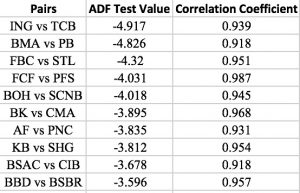
The following table demonstrates the top 10 selected pairs in the training period mentioned above. We can see that the pairs with the highest correlation coefficient doesn't necessarily have the best ADF test value. We made the rank by ADF test value because it's more robust.
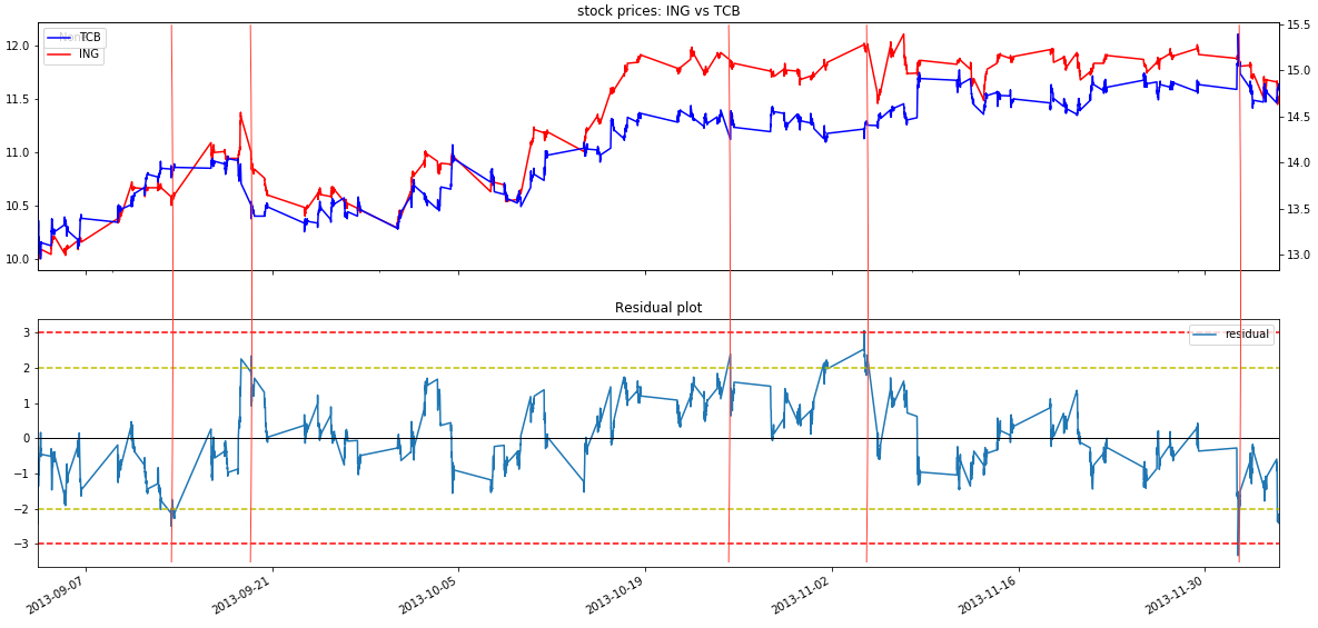
The upper part of the following chart plots the stock prices of pair ING vs TCB. The lower part plots by how many times standard deviation the residual deviate from its mean. There are 5 trading opportunities if we set the opening threshold to be 2.32.
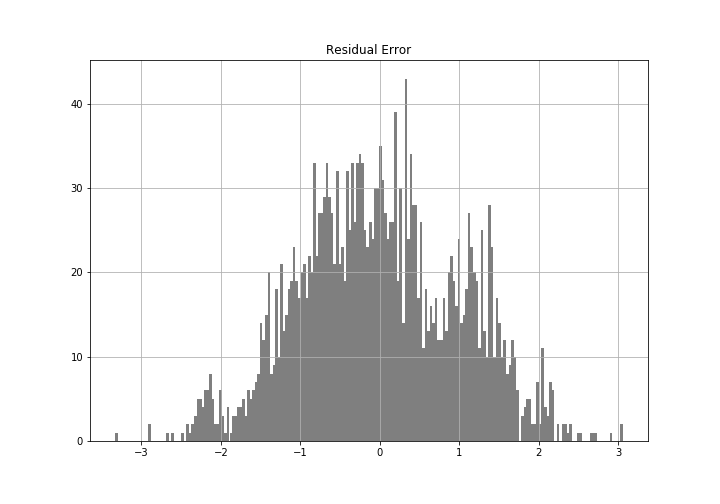
The following chart is the density plot of the residual error. From the shape we can see the error is approximately normal distributed.
Summary
The strategy is considered to be market neutral strategy because it a long/short strategy betting on price convergence. Out backtested beta is 0.232, which is within our expectation as a small value. Theoretically, the higher resolution we use, the higher win rate is because on one hand the higher resolution would increase the number of datapoint in our training period, which would make it's harder to past the two-stage test; on the other hand the higher resolution data would let us capture minor profit more accurately. However, there is a trade off between performance and backtesting time, as well as small size arbitrage profit versus transaction fee/friction. The higher resolution will lead backtesting time to increase drastically. The number of stocks in the initialize step would also affect our performance. Theoretically, the more stock we have, we better pairs we are likely to pick. But too many stocks would also be time consuming. what's worth mentioning is that the optimized parameters are different for each sector. It depends on the features of the price patterns in the specific industry. Plotting the pairs prices and the residual to observe is good option to adjust the thresholds.
Reference
- George J. Miao High Frequency and Dynamic Pairs Trading Based on Statistical Arbitrage Using a Two-Stage Correlation and Cointegration Approach Online Copy
- Cartea & Penalva, 2012, Where is the value in high frequency trading? Online Copy
- Gatev, Goetzmann, & Rouwenhorst, 2006, Pairs trading: Performance of a relative-value arbitrage rule. The Review of Financial Studies, 19(3), 797–827. Online Copy
- Engle and Granger, Co-integration and error correction: Representation, estimation, and testing. Econometrica, 55(2), 251–276. Online Copy


Pavel Fedorov
cloned and ran this code… it threw an error Error Message
During the algorithm initialization, the following exception has occurred: Trying to dynamically access a method that does not exist throws a TypeError exception. To prevent the exception, ensure each parameter type matches those required by the 'float'>) method. Please checkout the API documentation. at __init__ trade_bar = TradeBar(bar.Index[1] in SymbolData.py: line 19 at Initialize self.symbol_data[symbol] = SymbolData(self in main.py: line 38 No method matches given arguments for .ctor: (, , , , , , )
Stacktrace
Trying to dynamically access a method that does not exist throws a TypeError exception. To prevent the exception, ensure each parameter type matches those required by the 'float'>) method. Please checkout the API documentation. at __init__ trade_bar = TradeBar(bar.Index[1] in SymbolData.py: line 19 at Initialize self.symbol_data[symbol] = SymbolData(self in main.py: line 38 No method matches given arguments for .ctor: (, , , , , , )
The material on this website is provided for informational purposes only and does not constitute an offer to sell, a solicitation to buy, or a recommendation or endorsement for any security or strategy, nor does it constitute an offer to provide investment advisory services by QuantConnect. In addition, the material offers no opinion with respect to the suitability of any security or specific investment. QuantConnect makes no guarantees as to the accuracy or completeness of the views expressed in the website. The views are subject to change, and may have become unreliable for various reasons, including changes in market conditions or economic circumstances. All investments involve risk, including loss of principal. You should consult with an investment professional before making any investment decisions.
Ashutosh
While debugging the tickers in the code.There were 2 issues:
1) SCNB was delisted on 17th Nov 2011.
Reference:
2) There are some bar.volume data that is nan.
which caused a method mismatch for TradeBar which expected a float value at bar.volume but got nan.You can use simple nan techniques from data science to handle nan values like mean volume/ median volume/ external data source or any other nan handler logic.I have used a cheap technique to skip when volume equals nan to run the backtest.
The material on this website is provided for informational purposes only and does not constitute an offer to sell, a solicitation to buy, or a recommendation or endorsement for any security or strategy, nor does it constitute an offer to provide investment advisory services by QuantConnect. In addition, the material offers no opinion with respect to the suitability of any security or specific investment. QuantConnect makes no guarantees as to the accuracy or completeness of the views expressed in the website. The views are subject to change, and may have become unreliable for various reasons, including changes in market conditions or economic circumstances. All investments involve risk, including loss of principal. You should consult with an investment professional before making any investment decisions.
Derek Melchin
See the attached backtest for an updated version of the algorithm in PEP8 style.
The material on this website is provided for informational purposes only and does not constitute an offer to sell, a solicitation to buy, or a recommendation or endorsement for any security or strategy, nor does it constitute an offer to provide investment advisory services by QuantConnect. In addition, the material offers no opinion with respect to the suitability of any security or specific investment. QuantConnect makes no guarantees as to the accuracy or completeness of the views expressed in the website. The views are subject to change, and may have become unreliable for various reasons, including changes in market conditions or economic circumstances. All investments involve risk, including loss of principal. You should consult with an investment professional before making any investment decisions.
To unlock posting to the community forums please complete at least 30% of Boot Camp.
You can continue your Boot Camp training progress from the terminal. We hope to see you in the community soon!