Simple Linear Regression

Introduction

In finance and economics filed, most of the models are linear ones. We can see linear regression everywhere, from the foundation of the model portfolio theory to the nowadays popular Fama-French asset pricing model. It's very important to understand how linear regression works in order to have a comprehensive understanding of those theories.

If we are holding a stock, we must be curious about the relationship between our stock return and the market return. Let's say we hold Amazon stock on the first day of this year. In order to see the relation directly, we plot the daily return of our stock on the y-axis and plot the S&P 500 index daily return on the x-axis.

from datetime import datetime
qb = QuantBook()
tickers = ["AMZN", "SPY"]
symbols = [qb.AddEquity(ticker).Symbol for ticker in tickers]

# Get stock prices
history = qb.History(symbols, datetime(2017, 1, 1), datetime(2017, 6, 30), Resolution.Daily)
df = np.log(history.close.unstack(0)).diff().dropna()
df.columns = tickers
df.tail()

Time	AMZN	SPY
2017-06-24	0.002434	0.001193
2017-06-27	-0.009771	0.000658
2017-06-28	-0.017456	-0.008089
2017-06-29	0.013777	0.008911
2017-06-30	-0.014647	-0.008828

We successfully create a DataFrame contains the daily logarithm return of Amazon stock and S&P500. Now let's plot it:

import matplotlib.pyplot as plt
plt.figure(figsize = (15,10))
plt.scatter(df.SPY,df.AMZN)
plt.show()

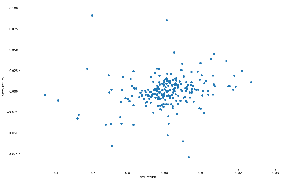
The plot is scattered, but we can see they are approximately correlated: generally the higher SPX's daily return is, the higher Amazon stock's return is. This is called positively correlated. We will cover it in the following tutorials.

Slope and Intercept

It's natural that we want to model the relation between these two rates of return. Intuitively we use a straight line to model it, this is called Linear Regression. In order to find the best straight line, it's natural to think that the vertical distances between the points of the data set and the fitted line should be minimized. Those vertical distances are called residual. Our objective is to make the sum of squared residuals as small as possible. This method is called ordinary least square, or OLS method. We use x and y to represent the two variable, S&P 500 daily returns and AMZN daily returns. The linear relation is:

$$Y = Y = \alpha + \beta*X + \epsilon$$

Where $\alpha$ is called intercept, $\beta$ is called slope. Generally, if the scatter points can be represented by ${(x_1,y_1),(x_2, y_2),(x_3,y_3)...(x_n,y_n)}$, then the intercept and slope are given by:

$$\beta = \frac{\sum_{i=1}^{n}(x-\bar{x})(y-\bar{y})}{\sum_{i=1}^{n}(x-\bar{x})^2}$$ $$\alpha = \bar{y} - \hat{\beta}\bar{x}$$

Where $\bar{x}$ is the mean of X, $\bar{y}$ is the mean of Y.

In python, we don't need to do the above calculation manually because we have package for it. But it still very important to understand the calculation process of $\beta$ in order the understand the modern portfolio theory and CAPM, which we will cover in the future.

Python Implementation

In python, we have a very power package for mathematical models, which is named 'statsmodels'.

import statsmodels.formula.api as sm
model = sm.ols(formula = 'AMZN~SPY',data = df).fit()
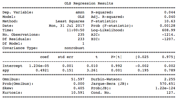
print(model.summary())

We built a simple linear regression model above by using the ols() function in statsmodels. The 'model' instance has lots of properties. The most commonly used one is parameters, or slope and intercept. We can access to them by:

print(f'pamameters: {model.params}')
[out]: pamameters: Intercept    0.001504
SPY          0.937181
dtype: float64
print(f'residual: {model.resid.tail()}')
[out]: residual: time
2017-06-24   -0.000189
2017-06-27   -0.011892
2017-06-28   -0.011379
2017-06-29    0.003921
2017-06-30   -0.007879
dtype: float64
print(f'fitted values: {model.predict()}')
[out]: fitted values: [ 7.06344221e-03  7.59665647e-04  4.85148106e-03 -1.59418889e-03 ... ]

Now let's have a look at our fitted line:

plt.figure(figsize = (15,10))
plt.scatter(df.SPY,df.AMZN)
plt.xlabel('spx_return')
plt.ylabel('amzn_return')
plt.plot(df.SPY,model.predict(),color = 'red')
plt.show()

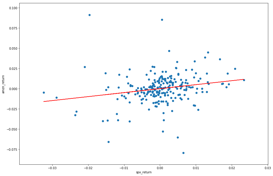
The red line is the fitted linear regression straight line. As we can see there are lot of statistical results in the summary table. Now let's talk about some important statistical parameters.

Parameter Significance

From the summary table we can see 'std err'. This means standard errors of the intercept and slope. The null hypothesis here is $H_0: \beta = 0$, and the alternative hypothesis is $H_1: \beta \neq 0$. This hypothesis score is calculated by:

$$t = \frac{\beta - 0}{SE}$$

Where SE is given by:

$$SE = \sqrt\frac{\frac{1}{n-2}\sum_{i = 1}^{n}\hat{\epsilon}^2}{\sum_{i = i}^{n}(x_i - \bar{x})^2}$$

The distribution used here is 'Student's t-distribution'. It's different from normal distribution but used in the similar way. The column 't' in this table is the test score, and 'p>|t|' is the p-value. By observing the p-value, we can see that the significance level of spy, or the slope, is very high because the p-value is close to zero. In other words, we have 99.999 confidence to claim that the slope is not 0, and there exists linear relation between X and Y. However, regarding the intercept, the p-value is 0.923, which means we have only 7.7% confidence level that the value of intercept is not 0. We can also see from the plot that the line crosses the origin. The following 2 columns are the lower band and upper band of the parameters at 95% confidence interval. At 95% confidence level, we can claim that the true value of the parameter is within this range.

Model Significance

Sum of Squared Errors, or SSE, is used to measure the difference between the fitted value and the actual value. It's given by: $$SSE = \sum_{i=1}^{n}(y_i - \hat{y_i})^2 = \sum_{i = 1}^{n}\hat{\epsilon_i}^2$$

If the linear model perfectly fitted the sample, the SSE would be zero. The reason we use squared error here is that the positive and negative errors would offset each other if we simply summed them up. Another measurement of the dispersion of the sample is called total sum of squares, or SS.. it's given by:

$$SS = \sum_{i = i}^{n}(y_i - \bar{y}_i)^2$$

If you are familiar with variance, we can see that SS divided by the number of sample n is the sample variance. From SSE and SS, we can calculate the Coefficient of Determination, or r-square for short. R-square means the proportion of variation that 'explained' by the linear relationship between X and Y, it's calculated by:

$$r^2 =1 = \frac{SSE}{SS} =1 - \frac{\sum_{i=1}^{n}(y_i - \hat{y_i})^2}{\sum_{i = i}^{n}(y_i - \bar{y}_i)^2}$$

Let's assume that the model perfectly fitted the sample, which means all of the sample points lie on the straight line. Then the SSE would become zero, and the r-square would become 1. This means perfect fitness. The higher r-square is, the more parts of variation can be explained by the linear relation, the higher significance level the model is.

Some other parameters, such as F-statistic, AIC and BIC, are related to multiple linear regression, with would be cover in the next chapter.

Summary

In this chapter we introduced how to implement simple linear in python, and focused on how to read the summary table. In next chapter we will introduced multiple linear regression, which are commonly used to built models in finance and economics.

---

---

---