Modern Portfolio Theory

Introduction

The Modern Portfolio Theory (MPT) suggests how investors should spread their wealth across various assets to minimize risk and maximize return.

This chapter is mathematically intense, so don't feel demoralized if you don't understand it on your first reading.

Risk Aversion

In portfolio theory, the riskiness of an asset is often measured by the variance (or standard deviation) of its returns. Risk-averse investors do not want their wealth to fluctuate wildly.

Risk aversion can be illustrated with a simple example. Which of the following assets do you prefer?

• Asset A pays $200 or $0 with 50% probability each.
• Asset B pays $400 or −$200 (i.e. you lose $200) with 50% probability each.

The expected payouts of A and B are:

$$\mathbb{E}(A) = 0.5 \times 200 + 0.5 \times 0 = 100$$ $$\mathbb{E}(B) = 0.5 \times 400 + 0.5 \times (-200) = 100$$

The standard deviation of their payouts are:

$$\sigma_A = \sqrt{0.5(200-100)^2 + 0.5(0-100)^2} = 100$$ $$\sigma_A = \sqrt{0.5(400-100)^2 + 0.5(-200-100)^2} = 300$$

If you are an risk seeker, you may choose asset B, because you can potentially get a higher payout. MPT assumes that investors prefer asset A since both assets have the same expected payout, but asset A has less risk.

Portfolio

Suppose we invest some fraction $w_1, w_2, \dots, w_n$ of our wealth in n risky assets (labelled 1 to n), and the remainder $w_0$ in a riskless asset such as cash in a bank account.

Clearly $w_0 + w_1 + \dots + w_n = 1$ since our wealth comprises all those assets.

Let $R_0, R_1, \dots, R_n$ be the respective asset returns, then our portfolio return is

$$R_P = w_0 R_0 + w_1 R_1 + \dots + w_n R_n$$

Alternatively, we can eliminate $w_0$ to get

$$R_P - R_0 = w_1 (R_1 - R_0) + \dots + w_n (R_n - R_0)$$

Our expected portfolio return is

$$\mathbb{E}(R_P) = w_0 R_0 + w_1 \mathbb{E}(R_1) + \dots + w_n \mathbb{E}(R_n)$$

Note that $\mathbb{E}(R_0) = R_0$ since the riskless return is known with certainty, by definition.

Correlation

Before computing portfolio risk, we need to first understand covariance and correlation. They measure the linear relationship between two random variables.

The covariance of two random variables X and Y is defined as

$$\text{Cov}(X, Y) = \mathbb{E} \left[ (X-\mathbb{E}(X)) (Y-\mathbb{E}(Y)) \right]$$

The correlation of X and Y, which is always between −1 and 1, is their covariance after being standardized:

$$\begin{equation} \begin{aligned} \text{Corr}(X, Y) &= \text{Cov} \left( \frac{X-\mathbb{E}(X)}{\sigma_X}, \frac{Y-\mathbb{E}(Y)}{\sigma_Y} \right) \\ &= \frac{\text{Cov}(X, Y)}{\sigma_X \sigma_Y} \end{aligned} \end{equation}$$

Risk

Now we are ready to compute portfolio risk, as measured by the variance of portfolio returns:

$$\text{Var}(R_P) = \text{Var}(w_0 R_0 + w_1 R_1 + \dots + w_n R_n)$$

Recall that $\text{Var}(X + c) = \text{Var}(X)$ if c is a known constant, so the term $w_0 R_0$ involving the riskless return can be omitted. It will be convenient to use sigma notation:

$$\text{Var}(R_P) = \text{Var} \left( \sum_{k=1}^n w_k R_k \right)$$ $$= \mathbb{E} \left[\left( \sum_{k=1}^n w_k R_k - \mathbb{E} \left( \sum_{k=1}^n w_k R_k \right) \right)^2\right]$$ $$= \mathbb{E} \left[\left( \sum_{k=1}^n w_k \, \left( R_k - \mathbb{E}(R_k) \right) \right)^2\right]$$

So we have a squared sum of n terms. How do we expand it?

$$\left( \sum_{k=1}^n u_k \right)^2 = (u_1 + \dots + u_n) \, (u_1 + \dots + u_n)$$

If we expand the brackets on the right hand side, every term has the form $u_i u_j$ where i and j can be 1, 2, ... , or n.

$$\left( \sum_{k=1}^n u_k \right)^2 = \sum_{i=1}^n \sum_{j=1}^n u_i u_j$$

Therefore

$$\begin{equation} \begin{aligned} \text{Var}(R_P) &= \mathbb{E} \left[ \sum_{i=1}^n \sum_{j=1}^n w_i \, w_j \, (R_i - \mathbb{E}(R_i)) (R_j - \mathbb{E}(R_j)) \right] \\ &= \sum_{i=1}^n \sum_{j=1}^n w_i \, w_j \, \text{Cov}(R_i, R_j) \end{aligned} \end{equation}$$

The last step arises from the definition of covariance. The only thing left is to express portfolio risk in matrix notation:

$$\text{Var}(R_P) = \mathbf{w}^T \Sigma \mathbf{w}$$

where

$$\mathbf{w} = \begin{pmatrix} w_1 \\ \vdots \\ w_n \end{pmatrix}$$ $$\Sigma = \begin{bmatrix} \text{Cov}(R_1, R_1) & \text{Cov}(R_1, R_2) & ... & \text{Cov}(R_1, R_n) \\ \text{Cov}(R_2, R_1) & \text{Cov}(R_2, R_2) & ... & \text{Cov}(R_2, R_n) \\ \vdots & \vdots & \ddots & \vdots \\ \text{Cov}(R_n, R_1) & \text{Cov}(R_n, R_2) & ... & \text{Cov}(R_n, R_n) \end{bmatrix}$$

Intuition

How can we make sense of portfolio risk? Consider a simple case with a riskless asset and only n = 2 risky assets.

$$\begin{equation} \begin{aligned} \text{Var}(R_P) &= w_A^2 \text{Var}(R_A) \\ &+ w_B^2 \text{Var}(R_B) \\ &+ 2w_A w_B \text{Cov}(R_A, R_B) \end{aligned} \end{equation}$$

Portfolio risk can be reduced by choosing two assets that are negatively correlated. This is the benefit of diversification.

Mean-Variance Analysis

We now try to find a portfolio $\mathbf{w} = (w_1, ..., w_n)$ that minimizes risk and maximizes return.

The chart below has risk (standard deviation of returns) on the horizontal axis and expected return on the vertical axis. The 10 black points represent individual stocks, while each green / blue point is a portfolio of stocks:

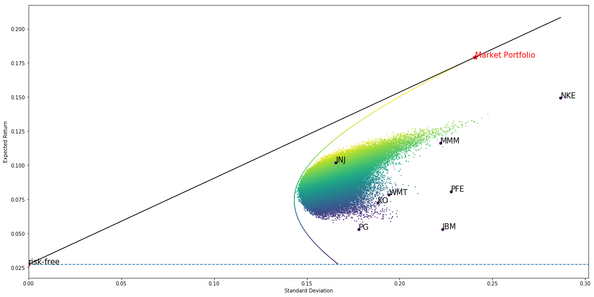
Notice that all points (i.e. stocks and portfolios) are enclosed by a hyperbola, known as the efficient frontier.

All portfolios on the efficient frontier have the maximum expected return for a given level of risk, if we only consider portfolios of risky stocks. Can we achieve higher returns by including a riskless asset? Yes.

Capital Market Line

The black line on the chart is the Capital Market Line (CML). It is tangent to the efficient frontier and cuts the vertical axis at the riskfree return. The point of tangency represents the so-called market portfolio.

Every point on the CML represents a portfolio comprising the market portfolio and riskless asset in some proportion. Why?

Suppose some fraction w of a CML portfolio is the market portfolio, and the remainder (1 − w) is the riskless asset. Then its expected return is

$$\mathbb{E} (R_P) = w \mathbb{E} (R_{\text{market}}) + (1-w) R_0$$

Since there is only n = 1 risky asset, the variance of the CML portfolio return is

$$\text{Var} (R_P) = w^2 \text{Var} (R_{\text{market}})$$

Taking square roots, we deduce that a CML portfolio's risk is proportional to the market portfolio's weight:

$$\sigma_P = w \sigma_{\text{market}}$$

This equation can be used to eliminate w in the calculation of expected return:

$$\mathbb{E} (R_P) = R_0 + \frac{\mathbb{E} (R_{\text{market}}) - R_0}{\sigma_{\text{market}}} \sigma_P$$

This proves that when $\mathbb{E} (R_P)$ is plotted against $\sigma_P$, we will obtain a straight line: the CML.

Portfolio Selection

Why is the CML significant? For any given level of risk, CML portfolios have a higher return than those on the efficient frontier, so investors should select any of them according to their risk tolerance.

Risk-averse investors may give the riskless asset a larger weight in their portfolio. Risk-seeking investors may borrow money (i.e. sell the riskless asset) to invest >100% of their wealth in the market portfolio.

Regardless of their risk tolerances, all investors should hold the same stocks in the same proportion in the market portfolio. In other words, they should not pick stocks according to their risk tolerance.

Diversification

What happens to the efficient frontier and hence the CML if we have only 3 stocks (IBM, GE, and PFE) instead of 10?

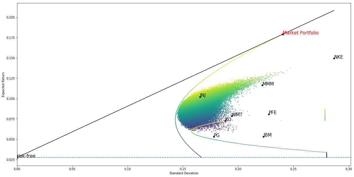
Since we have fewer stocks to choose from, it's not too surprising that our maximum expected return is lower for any level of risk. This demonstrates why diversification is often said to be a "free lunch" in investing.

Summary

In this chapter we have learnt about the modern portfolio theory. It recommends investors to spread their wealth across many asset classes to maximize returns while minimizing risk. In the next chapter, we will introduce the Capital Asset Pricing Model.

---

---

---