Market Risk

Introduction

In the financial literature, you may hear terms like the "beta" or "market risk" of an asset. This chapter will explain where these terms come from and how they can be useful.

Capital Asset Pricing Model

As we shall see later, the name "Asset Pricing" is a bit misleading because the CAPM tells us the expected return, rather than the price, of an asset. In the last chapter, we introduced the Capital Market Line (CML) shown in black:

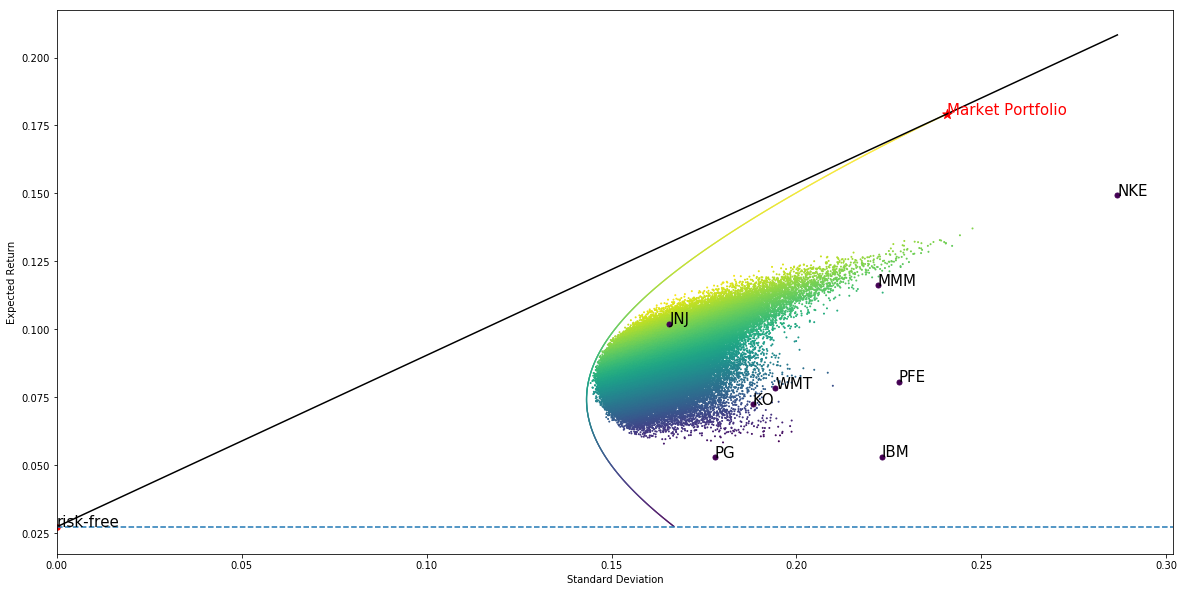
All investors should hold a portfolio on the CML, which is constructed by investing some fraction w of our wealth in the market portfolio and the remainder (1 − w) in the riskless asset. So the return on a CML portfolio is

$$R = w R_{\text{market}} + (1-w) R_0$$

If we let β = w, then the equation above becomes

$$R - R_0 = \beta (R_{\text{market}} - R_0)$$

Notice that β is a measure of how sensitive our CML portfolio return is to the market return. Taking expectation on both sides results in the CAPM:

$$\mathbb{E}(R) - R_0 = \beta (\mathbb{E} (R_{\text{market}}) - R_0)$$

Taking covariance on both sides instead yields

$$\text{Cov} (R - R_0, R_{\text{market}}) = \beta \text{Cov} (R_{\text{market}} - R_0, R_{\text{market}})$$

Now apply two basic facts about covariance:

• $\text{Cov} (X + c, Y) = \text{Cov} (X, Y)$ where $c$ is constant
• $\text{Cov} (X, X) = \text{Var} (X)$

Hence we obtain

$$\beta = \frac {\text{Cov} (R, R_{\text{market}})} {\text{Var} (R_{\text{market}})}$$

Computing beta in Practice

While the Capital Asset Pricing Model is straightforward, applying it may not be. We first need to choose the timeframe for computing returns: should we use daily, weekly or monthly returns? Then we need to consider the number of data points available for linear regression. For example, if we compute beta using monthly returns in the past 1 year, then we only have 12 data points which is too few.

Furthermore, the β of an asset can change over time. The following plot is the daily rolling beta of GE stock with a 6-month rolling windows:

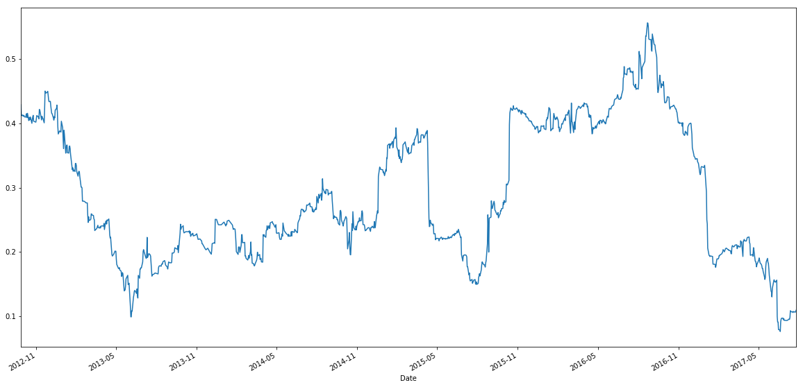
The β of GE ranged from 0.1 to 0.5 approximately. This is why you need to be careful when using β. It makes no sense to talk about β without a timeframe in mind.

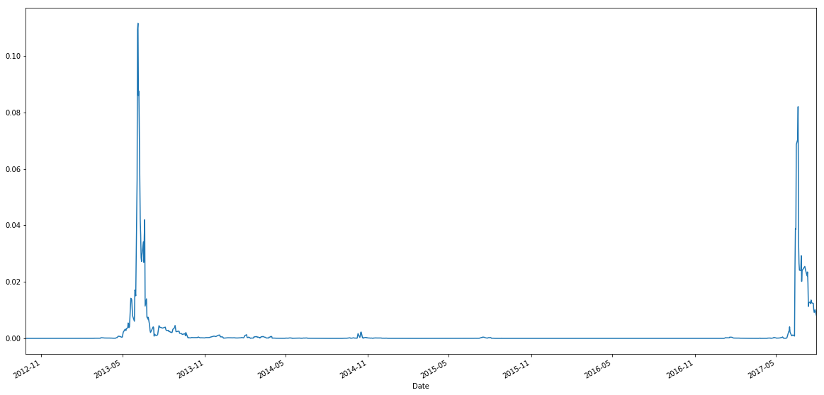
The following graph is the rolling p-value of beta. The p-value stays close to zero most of the time. However, during some period it suddenly increased close to 0.1, which corresponds to a 90% confidence interval. This might be caused by some mispricing or market turmoil.

Market-Neutral

A portfolio is market-neutral if its β is zero. In other words, the portfolio's returns are uncorrelated with market returns. We say that it has no "market risk". Some classical market-neutral strategies are pairs trading, beta-hedged equity portfolio and other derivatives strategies.

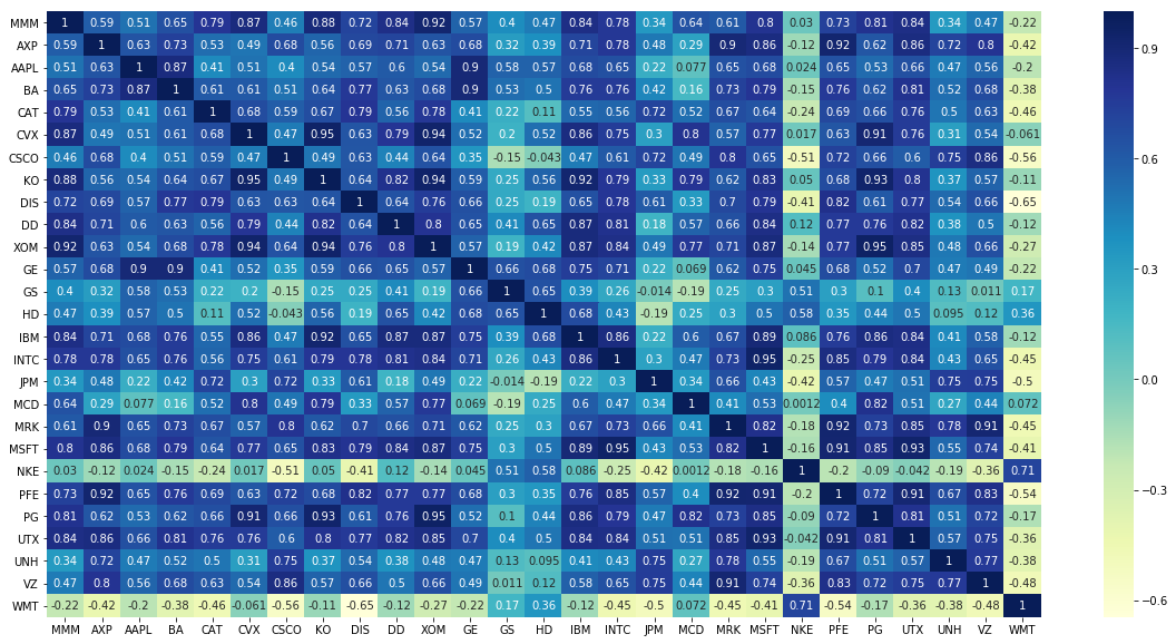
We have daily returns of Dow 30 stocks from March 2012 to Jan 2015. For each stock, its β on any given day is computed using the past 6 months' returns. As this 6-month window moves forward in time, β will of course change.

Once we know how each stock's β has changed over time, we can ask: which stocks' betas are correlated with each other? The table below shows the correlation between each stock's beta.

How can we construct a market-neutral portfolio? Consider two stocks A and B:

$$R_A = R_0 + \beta_A (R_{\text{market}} - R_0)$$ $$R_B = R_0 + \beta_B (R_{\text{market}} - R_0)$$

Let's allocate w on stock A and (1 − w) on stock B, then market neutrality means

$$\begin{equation} \begin{aligned} w\beta_A + (1-w) \beta_B &= 0 \\ \Rightarrow w &= \frac{\beta_B}{\beta_B - \beta_A} \end{aligned} \end{equation}$$

As mentioned earlier, $\beta_A$ and $\beta_B$ will change with time, so will $w$ in a market-neutral portfolio. However we can achieve market neutrality with constant $w$ so long as $\beta_A$ and $\beta_B$ have a linear relationship:

$$\beta_A = m\beta_B + c$$

Then eliminate $\beta_A$ to get

$$w = \frac{\beta_B}{(1-m) \beta_B - c}$$

If c &approx 0 then w is roughly constant:

$$w = \frac{1}{1-m}$$

Note: If c is signficant, then we need 3 stocks to get zero net beta. Usually 2 stocks are sufficient to cancel out most of the market risk.

Example

The 6-month rolling betas of PG and KO stocks have a correlation of 93%. The linear relationship between their betas is

$$\beta_{KO} = -0.0097 + 0.969 \beta_{PG}$$

Therefore the market neutral weights are

$$\begin{equation} \begin{aligned} w_{KO} &= \frac{1}{1-0.969} = 32.3 \\ w_{PG} &= 1 - w_{KO} = -31.3 \end{aligned} \end{equation}$$

We tested this portfolio both in-sample (March 2012 to Jan 2015) and out-of-sample. It achieved a beta of 0.01 and -0.004 respectively. See the backtest below.

Summary

This chapter has explained what market risk means in the context of CAPM, and how market risk can be reduced. In the next chapter we will generalize CAPM to multi-factor models, such as the Fama-French models.

---

---

---