Intraday Application of Hidden Markov Models

Introduction

A Hidden Markov Model (HMM) estimates the probability an asset will continue similar behavior or jump to another state, making it a great tool to predict the current market regime (trending up, ranging, or trending down). In this micro-study, we implement a 3-component HMM strategy to detect market regimes and generate timely buy signals for liquid stocks on an intraday basis.

Background

A HMM is a probabilistic model representing a sequence of events or observations, where the underlying process that generates the observations is not directly observable. 

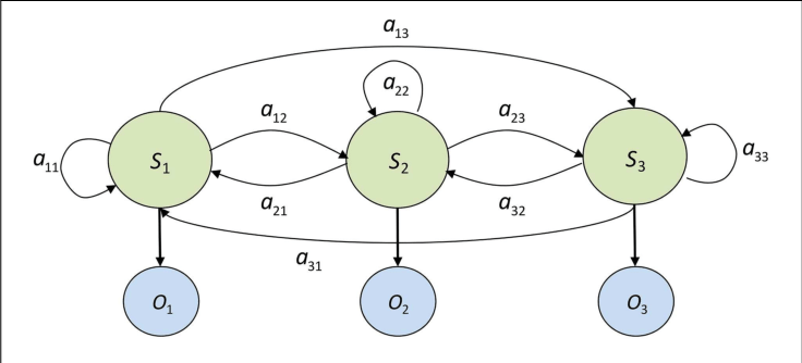
The use of HMMs in financial market analysis has gained traction in recent years. HMMs are powerful statistical models that can effectively capture the underlying, unobservable market states or "regimes" that drive asset price movements.

Their only input is price, so we wanted to focus on intraday timeframes to reduce the impact of the economy, politics and other macro factors.  To start we chose 5-minute close price returns of the top 10 market cap stocks. These stocks tend to be highly liquid and less volatile, making them suitable for a rapid, intraday trading strategy. The 5-minute bar timeframe was sufficient to identify market regime shifts while maintaining a rapid response to intraday market fluctuations.

Implementation

To implement this on QuantConnect, we used universe selection, a data consolidator, and a returns indicator. 

1. First, the strategy selects the top 10 US stocks by market capitalization. This is a fairly stable list as the top-10 don't change very frequently. By default this subscribes at minute resolution and updates daily. 

def initialize(self):
    self.add_universe(lambda fundamental: [f.symbol for f in sorted(fundamental, key=lambda x: x.market_cap, reverse=True)[:10]])

2. We create a HMM object for the assets added to the algorithm, and set the random seed state to ensure the backtest result is repeatable. To remember the training state of the model we've created a model_month flag.

def on_securities_changed(self, changes):
    for added in changes.added_securities:
        added.model = hmm.GaussianHMM(n_components=3, n_iter=100, random_state=100)
        added.model_month = -1

3. Then we consolidate the minute data, and pipe the 5-minute bars into the on_consolidated event handler. We also create the rate-of-change indicator which will record the history of returns for our model.

added.roc = RateOfChange(1)
added.roc.window.size = 150
added.consolidator = TradeBarConsolidator(timedelta(minutes=5))
added.consolidator.data_consolidated += self.on_consolidated
self.subscription_manager.add_consolidator(added.symbol, added.consolidator)

4. Later, when five minute bars are produced, we update the RateOfChange indicator. This automatically adds new return values to its rolling window, building the training data for our model. When we have enough data, the model is trained on the points available.

def on_consolidated(self, _, bar):
	security = self.securities[bar.symbol]
	security.roc.update(bar.end_time, bar.price)
	if security.roc.window.is_ready:
		if security.model_month != bar.end_time.month:
			security.model.fit(np.array([point.value for point in security.roc.window])[::-1].reshape(-1, 1))
			security.model_month = bar.end_time.month

5. The model can then use the latest 5-minute return to predict the current market regime for each asset. If P(positive) > P(negative), buy the stock, else short sell it. We use a fixed weight of 10% to ensure equal exposure.

post_prob = security.model.predict_proba(np.array([security.roc.current.value]).reshape(1, -1)).flatten()
self.set_holdings(bar.symbol, 0.1 if post_prob[2] > post_prob [0] else -0.1)

Results

The implementation of a three-component Hidden Markov Model strategy for the top 10 market capitalization stocks yielded exceptional performance, with a Sharpe Ratio of 1.9. The model could quickly identify market regimes and capitalize on shifts in market conditions. By using a universe of liquid stocks we could efficiently trade intraday, and  place multiple concurrent bets to smooth the overall return.

The algorithm parameter values (5, 150) were chosen at random. The strategy was resilient to a wide range of different parameters with all tests falling between 1.1-1.9 Sharpe Ratio.

As with any investment strategy, ongoing monitoring, optimization, and risk management practices are essential to maintain robust performance over time.