Research

Machine learning algorithms provide another way to analyze and conduct research on data. They allow us to detect patterns on large datasets and create predictive models. There are many machine learning libraries which make it easy to create, train and use various machine learning models. QuantConnect supports many of the popular frameworks like SciKit and TensorFlow. You can find a full list of the supported libraries in the Machine Learning documentation.

Scikit-learn is a framework that provides us with many ready to use algorithms for classification and regression, like support vector machines (SVM), random forests, and many more. SciKit is great to use if you want to quicky test an idea or hypothesis using a machine learning algorithm, without having to worry about building a model from the ground up.

Linear Regression Example

Regression uses past data to train a model that can predict future data. There are many different regressions with various degrees of sophistication. Linear regression is one of the simple of these models. Linear regression aims to create a linear approximation of future data. Scikit provides the LinearRegression method which creates a ready to go regression model for us to train and use.

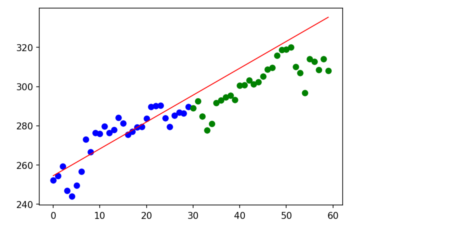
Let's create a linear regression model trained on 30 days of historical SPY price data and use to predict the next 30 days of data. We'll need to first import our dependencies from SciKit and subscribe to SPY data.

from sklearn.linear_model import LinearRegression

qb = QuantBook()
spy = qb.AddEquity("SPY") 

Next, let's make a history call for the last 60 days of price data. We will use the first 30 days to train our model and then use the next 30 days to test our model.

# 60 days of SPY data
spy_history = qb.History(spy.Symbol, 60, Resolution.Daily)

# Drop the symbol index from multi-index dataframe
spy_history = spy_history.reset_index(level=0, drop=True)

# Get list of 60 days of open prices from dataframe
prices = list(spy_history['open'])

The linear regression model requires two series, train_X and train_Y, to train our model with. We want to predict prices using our model so the prices will be our train_Y. We can use a time series starting at t=0 as our train_X.

# Create time series list of training range
train_range = range(30)

# Format time series data into form compatible with LinearRegression
train_X = np.column_stack([np.ones(len(A)), A])

# First 30 days of price data used for training
train_Y = price[:30]

# Define LinearRegression model from scikit
reg = LinearRegression()

# Fit model with training data
reg.fit(train_X, train_Y)

Now we can test the model's predictions on the next 30 days of data against the actual prices. First, we create a test_X for the entire 60 days of time, then feed the model with it and save its predictions.

# 60 day time series
test_range = range(60)

# Format time series data
test_X = np.column_stack([np.ones(len(test_range)), test_range])

# Use linear regression model to predict prices
prices_pred = reg.predict(test_X)

To visualize how well our model performs, we can plot the price data overlayed with the linear model. Let's split the price data scatter plot into two sections, blue for our training data and green for our testing data.

# The first 30 days of price data used to train model
plt.scatter(test_range[:30], prices[:30], color='blue')

# The next 30 days of price data
plt.scatter(test_range[30:60], prices[30:60], color="green")

# The linear regression model
plt.plot(test_range, prices_pred, color='red', linewidth=1)

TensorFlow is a low-level library that we can use to implement machine learning algorithms. Unlike scikit, TensorFlow does not have any ready to use algorithms, Instead, TensorFlow provides the building blocks to implement the algorithms we need. TensorFlow is especially great for implement deep learning algorithms and working with large datasets since it allows us to take advantage of GPU's for training our models.

Preparing Data For Training and Testing

Let's create a neural network that predicts future prices given past prices. We'll build our network with TensorFlow and then train it using historical data. We can then test our model by visualizing its predictions against actual historical prices. First, we'll need to retrieve historical data for SPY.

import tensorflow as tf

qb = QuantBook()
spy = qb.AddEquity("SPY").Symbol

# retrieve close data
data = qb.History(spy, 
                  datetime(2020, 6, 22), 
                  datetime(2020, 6, 27), 
                  Resolution.Minute).loc[spy].close

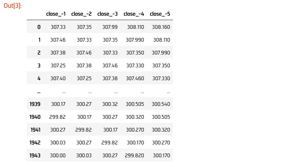
We'll feed our network the last 5 close prices to predict the next close. Let's format our data into our input dataframe X by offsetting our historical close prices.

# Feeding 5 input past prices to predict the next price
lookback = 5
# Series to hold each set of input prices
lookback_series = []

# Offsetting close data by length of lookback
for i in range(1, lookback + 1):
    df = data.shift(i)[lookback:-1]
    df.name = f"close_-{i}"
    lookback_series.append(df)

# Formatting offset data into input format
X = pd.concat(lookback_series, axis=1).reset_index(drop=True)

Since we'd like to predict the closing price of SPY 1 timestep into the future, we should create a dataframe containing this data. This will serve as our neural network's training and testing output Y.

# Shift our time series close data by 1
Y = data.shift(-1)[lookback:-1].reset_index(drop=True)

We can then split our data into training and testing sets using scikit-learn's train_test_split. We will use the training set to train our model and then assess the network's predictions against the test data. Let's use a third of our data to test and the remaining to train our model.

# import scikit-learn's train_test_split method
from sklearn.model_selection import train_test_split

# split historical data into training and testing sets
X_train, X_test, y_train, y_test = train_test_split(X, Y, test_size=0.33, shuffle=False)

Building Models

Let's build a neural network with 3 hidden layers and an output layer. We'll have 32 neurons in our first layer, 16 in our second, and 8 in our third layer.

# Initialize a tensorflow graph object
tf.reset_default_graph()
sess = tf.Session()

# parameters for our neural network
num_factors = X_test.shape[1]
num_neurons_1 = 32
num_neurons_2 = 16
num_neurons_3 = 8

# Placeholders for our inputs and outputs
X = tf.placeholder(dtype=tf.float32, shape=[None, num_factors], name='X')
Y = tf.placeholder(dtype=tf.float32, shape=[None])

Next, we can build our model layer by layer. We will need a set of weights and biases for each layer.

# Initializers
weight_initializer = tf.variance_scaling_initializer(mode="fan_avg", distribution="uniform", scale=1)
bias_initializer = tf.zeros_initializer()

# Hidden weights
W_hidden_1 = tf.Variable(weight_initializer([num_factors, num_neurons_1]))
bias_hidden_1 = tf.Variable(bias_initializer([num_neurons_1]))
W_hidden_2 = tf.Variable(weight_initializer([num_neurons_1, num_neurons_2]))
bias_hidden_2 = tf.Variable(bias_initializer([num_neurons_2]))
W_hidden_3 = tf.Variable(weight_initializer([num_neurons_2, num_neurons_3]))
bias_hidden_3 = tf.Variable(bias_initializer([num_neurons_3]))

# Output weights
W_out = tf.Variable(weight_initializer([num_neurons_3, 1]))
bias_out = tf.Variable(bias_initializer([1]))

# Hidden layer
hidden_1 = tf.nn.relu(tf.add(tf.matmul(X, W_hidden_1), bias_hidden_1))
hidden_2 = tf.nn.relu(tf.add(tf.matmul(hidden_1, W_hidden_2), bias_hidden_2))
hidden_3 = tf.nn.relu(tf.add(tf.matmul(hidden_2, W_hidden_3), bias_hidden_3))

# Output layer
output = tf.transpose(tf.add(tf.matmul(hidden_3, W_out), bias_out), name='outer')

Training Models

We will need a loss function and an optimizer function to train our model; we can use TensorFlow's built-in tf.squared_difference and tf.train.AdamOptimizer(), respectively. An epoch is an iteration of our entire training set. Let's train our model for 20 epochs.

 # Define loss and optimizer functions
loss = tf.reduce_mean(tf.squared_difference(output, Y))
optimizer = tf.train.AdamOptimizer().minimize(loss)
sess.run(tf.global_variables_initializer())

# Define training parameters
batch_size = len(y_train) // 10
epochs = 20

# Train Model
for _ in range(epochs):
    for i in range(0, len(y_train) // batch_size):
        start = i * batch_size
        batch_x = X_train[start:start + batch_size]
        batch_y = y_train[start:start + batch_size]
        sess.run(optimizer, feed_dict={X: batch_x, Y: batch_y}))

Testing Models

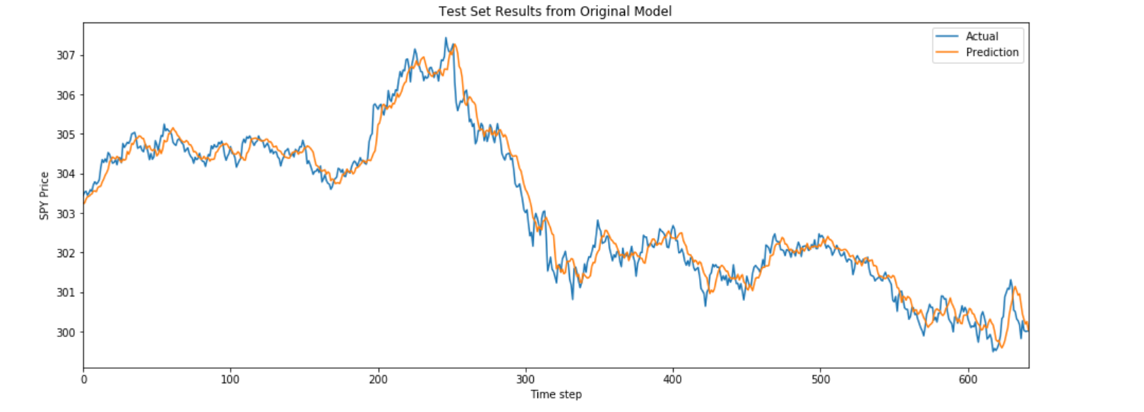
Finally, let's test how accurate our model is by plotting its predictions against actual price data.

prediction = sess.run(output, feed_dict={X: X_test})
prediction = prediction.reshape(prediction.shape[1], 1)
y_test.reset_index(drop=True).plot(figsize=(16, 6), label="Actual")

# Plot predictions
plt.plot(prediction, label="Prediction")
plt.title("Test Set Results from Original Model")
plt.xlabel("Time step")
plt.ylabel("SPY Price")
plt.legend()
plt.show()

Keras is a high level library for neural networks. Keras was designed to be modular fast and easy to use. It allows for easy and quick implementations of models.

Neural networks provide a way to predict future prices based on past prices. In order to accomplish this in Keras, we will need to create a Sequential model and train it with historical data. After our model has been trained, we can test its accuracy by comparing its predictions against historical prices. First, let's import the necessary dependencies and subscribe to SPY data.

from keras.models import Sequential
from keras.layers import Dense, Flatten
from keras.optimizers import RMSprop

spy = qb.AddEquity("SPY")

Preparing Data For Training and Testing

Let's create a model that predicts the next percent change in closing price given 5 days of OHLCV data. We can make a history call for 360 days of data that we will use to both train and test our model.

spy_hist = qb.History(qb.Securities.Keys, 360, Resolution.Daily).loc['SPY']

# n_tsteps is the number of time steps at and before time t we want to use
# to predict the close price at time t + 1
# in this case it is 5
n_tsteps = 5

# this helps normalizes the data
df = data.pct_change()[1:]
    
features = []
labels = []

# Format data into inputs/features and outputs/labels
for i in range(len(df)-n_tsteps):
    input_data = df.iloc[i:i+n_tsteps].values
    features.append(input_data)
    label = df['close'].iloc[i+n_tsteps]
    labels.append(label)

X, y = np.array(features), np.array(labels)

Now we can split our historical data into training and testing sets. We'll use the first 300 days of data to train our model and the remaining days to test our model.

# split data into training/testing sets
X_train = X[:300]
X_test = X[300:]
y_train = y[:300]
y_test = y[300:]

Building Models

Next, we create our neural network model. The Keras Sequential model allows us to create a neural network layer by layer. We will use a neural network with 2 hidden layers and a flatten layer, which is required because our input data is 2-dimensional; i.e. there are 5 input days, each with OHLCV data. We'll use a mean-square error loss function with an RMSprop optimizer function.

model = Sequential([
        # 5 input variables (OHLCV) by 5 time steps
        Dense(10, input_shape=(5,5), activation='relu'),
        Dense(10, activation='relu'),

        # Flatten layer required because input shape is 2D
        Flatten(),

        # since we are performing regression, we only need 1 output node
        Dense(1)
    ])

# Set loss function and optimizer
model.compile(loss='mse',
                optimizer=RMSprop(0.001),
                metrics=['mae', 'mse'])

Training and Testing Models

Keras allows for easy training using the model.fit(x_train, y_train, epochs) method. This method iterates through our training set once for each epoch.

# Train model with training data
model.fit(X_train, y_train, epochs=5)

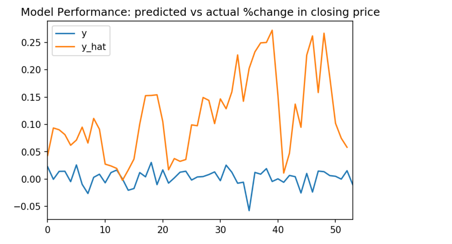
Finally, let's visualize our neural networks accuracy by plotting its predictions alongside the historical prices changes. We can use model.predict(x_test) to retrieve our model's predictions on the test set. Then we can format our predicted prices and actual historical changes in a dataframe, and plot that dataframe.

y_hat = model.predict(X_test)
df = pd.DataFrame({'y': y_test.flatten(), 'y_hat': y_hat.flatten()})
df.plot(title='Model Performance: predicted vs actual %change in closing price')

Training machine learning algorithms can be quite computationally expensive. There is a 10 minute limit on a time single loop in backtesting. This means that if we are training a model on a large dataset, algorithm may time out. The self.Train method increases this limit to 30 minutes, allowing us more time to train our model. You can learn more in the Machine Learning documentation.

The Object Store is a project specific storage space available in the QuantConnect web environment. We can use the Object Store to save trained models for future use. You can learn more about the Object Store in the Machine Learning documentation.

Keras

In order to save our model, we can first use serialize_keras_object from the keras.util library to convert our model into a json. Then we can convert our json into string using json.dumps. Finally, we save our model using qb.ObjectStore.Save. We will need to provide the Object Store a key to reference our saved object.

model_key = 'my_model'
import json
from keras.utils.generic_utils import serialize_keras_object

modelStr = json.dumps(serialize_keras_object(model))
qb.ObjectStore.Save(model_key, modelStr)

Then we can load our model from the Object Store using qb.ObjectStore.Read with our key. We should make sure our key exists in the Object Store before attempting to access it. Then we can convert our string back into a json and finally create a sequential model from it using Sequential.from_config.

if qb.ObjectStore.ContainsKey(model_key):
    modelStr = qb.ObjectStore.Read(model_key)
    config = json.loads(modelStr)['config']
    model = Sequential.from_config(config)