Research

Fundamental data includes revenues, earnings, profit margins, and other data, which allows us determine a company's underlying value and potential for future growth. QuantConnect provides fundamental data from MorningStar for over 5000 US equities going back as far as 1998. There are over 900 different data fields, including earning reports, income statements and more. You can find a list of all the available fields in the data library.

Making History Calls

We can directly access fundamental data for a given data field using qb.GetFundamental(Symbols, Selector, StartDate, EndDate). Symbols is the list of symbols that interest us. Selector is the name of the fundamental data field. If StartDate and EndDate are not specified, QuantBook will get all the fundamental data starting from January 1st, 1998. In order to access fundamental data, we will first need to subscribe to some symbols.

qb = QuantBook()
aapl = qb.AddEquity("AAPL")
amzn = qb.AddEquity("AMZN")
goog = qb.AddEquity("GOOG")
ibm = qb.AddEquity("IBM")

For some quarterly or yearly reported fundamentals like FinancialStatements and OperationRatios, we need to specify the period at the end of the fundamental selector name. For example, EarningReports.BasicAverageShares.TwelveMonths gives us the one year value of the basic average shares, while EarningReports.BasicAverageShares.ThreeMonths gives us the three month value,.

start_time = datetime(2017, 1, 4) # January 4th 2017
end_time = datetime.now() # Today's date

# Get the PE ratio for all securities between given dates
pe_history = qb.GetFundamental(qb.Securities.Keys, "ValuationRatios.PERatio", start_time, end_time)

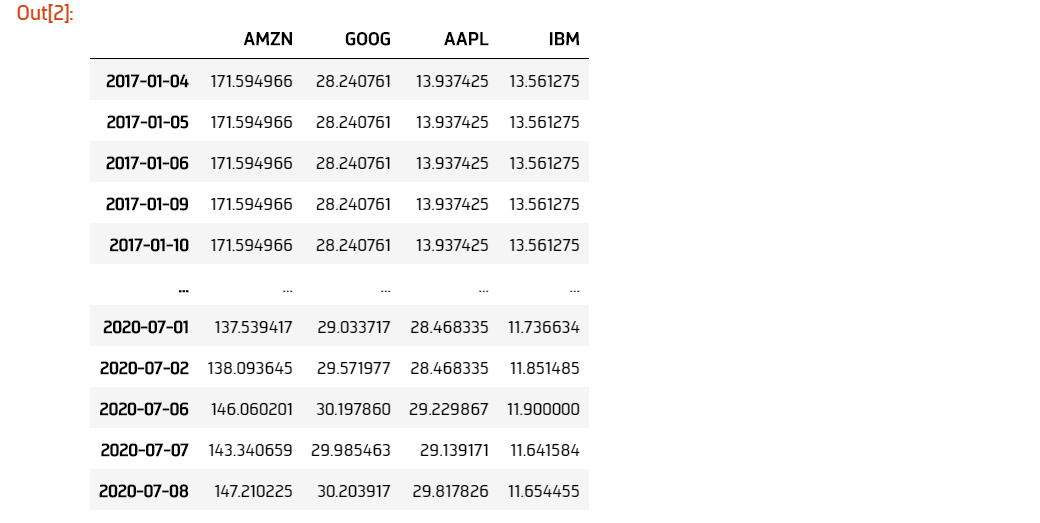
# Get the AAPL yearly EBITDA since 1998
ebitda_history = qb.GetFundamental([aapl.Symbol, goog.Symbol], "FinancialStatements.IncomeStatement.EBITDA.TwelveMonths")

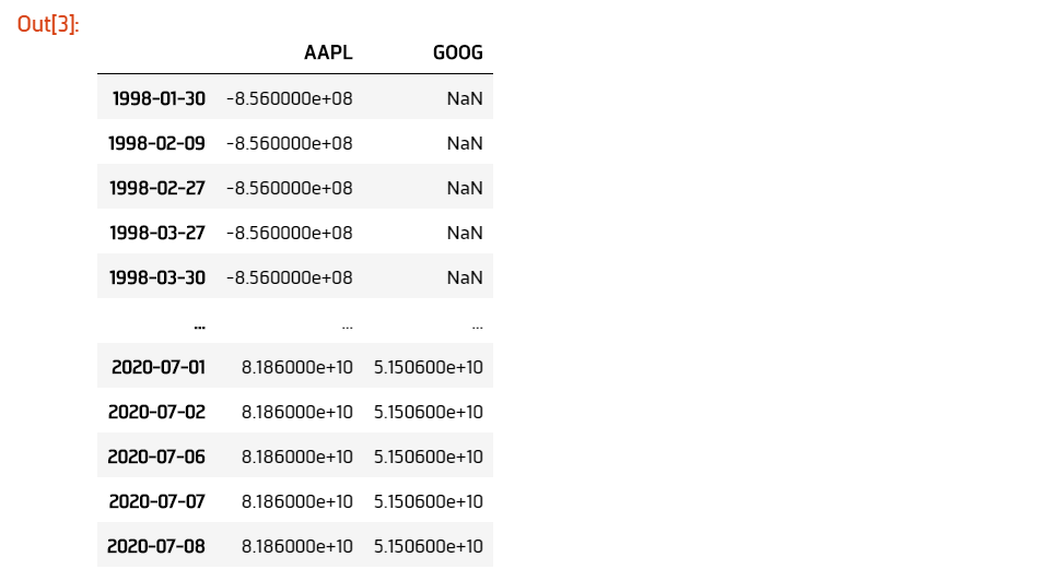
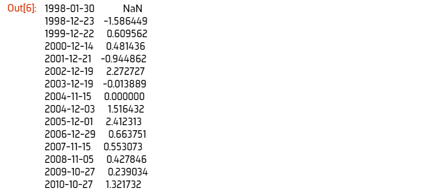
Notice that the values for GOOG are NaN for the years before GOOG's IPO.

Accessing and Manipulating Data

For history calls on multiple symbols, we can access the data for a specific symbol.

# Get the EBITDA history for AAPL
aapl_ebitda = ebitda_history['AAPL']

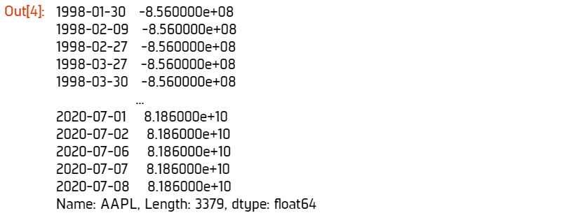
Since the history call returns daily resolution data and the twelve-month EBITDA is updated yearly, there will be duplicate data points in our dataframe. We can remove the duplicate points and look at the unique EBITDA entries.

# drop duplicate EBITDA Values
aapl_ebitda_filtered = aapl_ebitda.drop_duplicates()

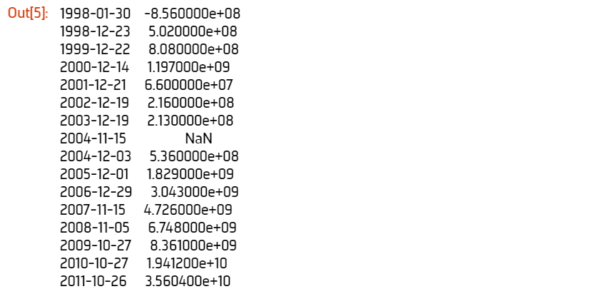
We can then calculate the year on year change of AAPL's EBITDA and assign the values to a new column change.

# Calculate YoY percent change of EBITDA
aapl_ebitda_filtered['change'] = aapl_ebitda_filtered.pct_change()

Example 1: Finding Undervalued Stocks

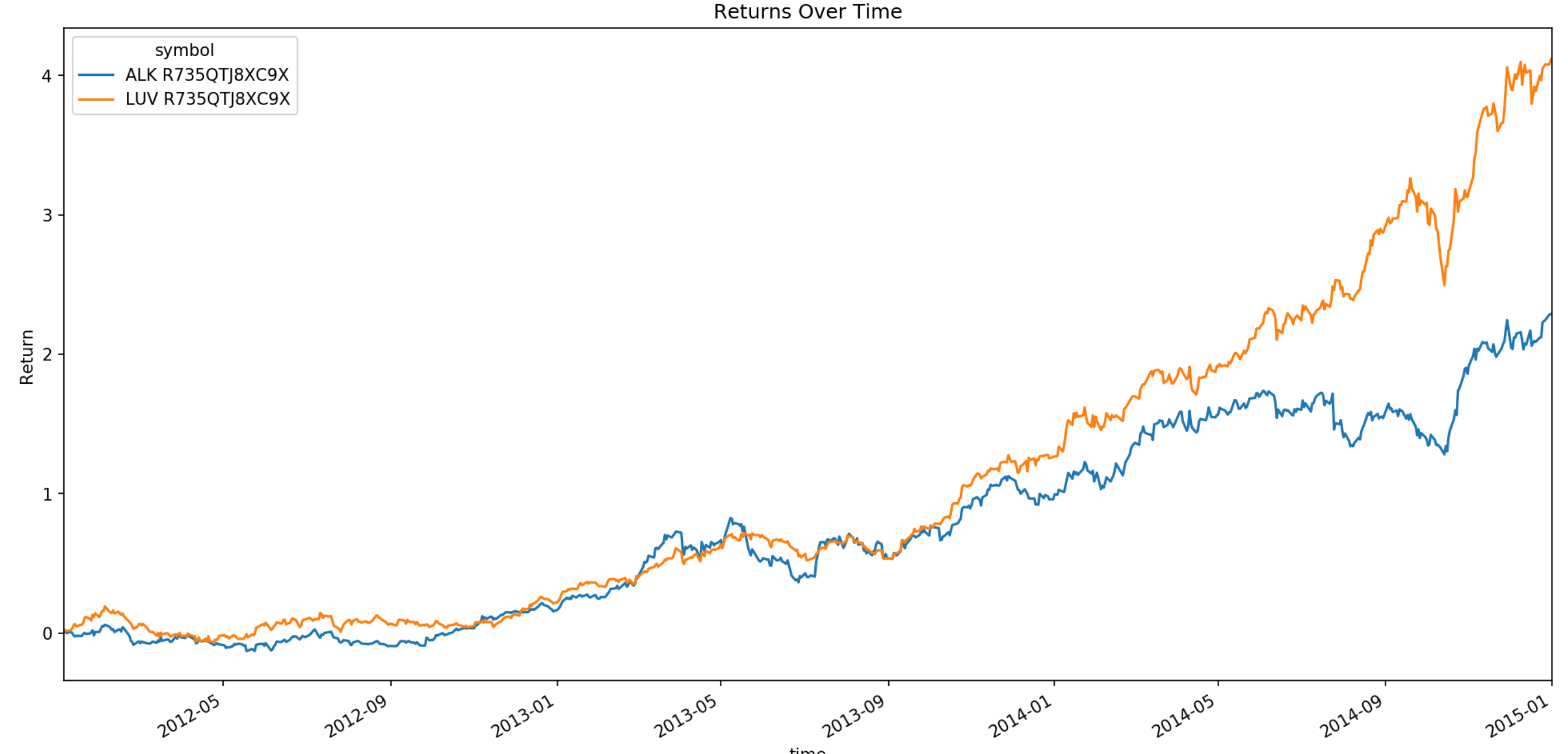
The Price-to-Earnings ratio is a measure of how expensive a company is relative to its earnings. PE ratios tend be to vary amongst industries as each industry has different operating costs and profit margins. We can find undervalued stocks by comparing its PE ratio to that of its industry. Stocks will a lower PE ratio than the industry average may be undervalued. Let's conduct an analysis on the airline industry and determine whether low PE ratio stocks outperform stocks with high PE ratios .

First let's subscribe to data for a set of airline stocks.

qb = QuantBook()

tickers = [
    "ALK",  # Alaska Air Group, Inc.
    "AAL",  # American Airlines Group, Inc.
    "DAL",  # Delta Air Lines, Inc.
    "LUV",  # Southwest Airlines Company
    "UAL",  # United Air Lines
    "ALGT", # Allegiant Travel Company
    "SKYW"  # SkyWest, Inc.
]

symbols = [qb.AddEquity(ticker, Resolution.Daily).Symbol for ticker in tickers]

Using qb.GetFundamental we can retrieve the PE ratios of these stocks over 2011. Let's then plot the PE ratios over that year to visualize how they vary.

# Request PE ratio data from 2014
pe_ratios = qb.GetFundamental(symbols, 
                              "ValuationRatios.PERatio", 
                              datetime(2014, 1, 1),
                              datetime(2015, 1, 1))

# Plot PE ratios
pe_ratios.plot(figsize=(16, 8), title="PE Ratio Over Time")
plt.xlabel("Time")
plt.ylabel("PE Ratio")
plt.show()

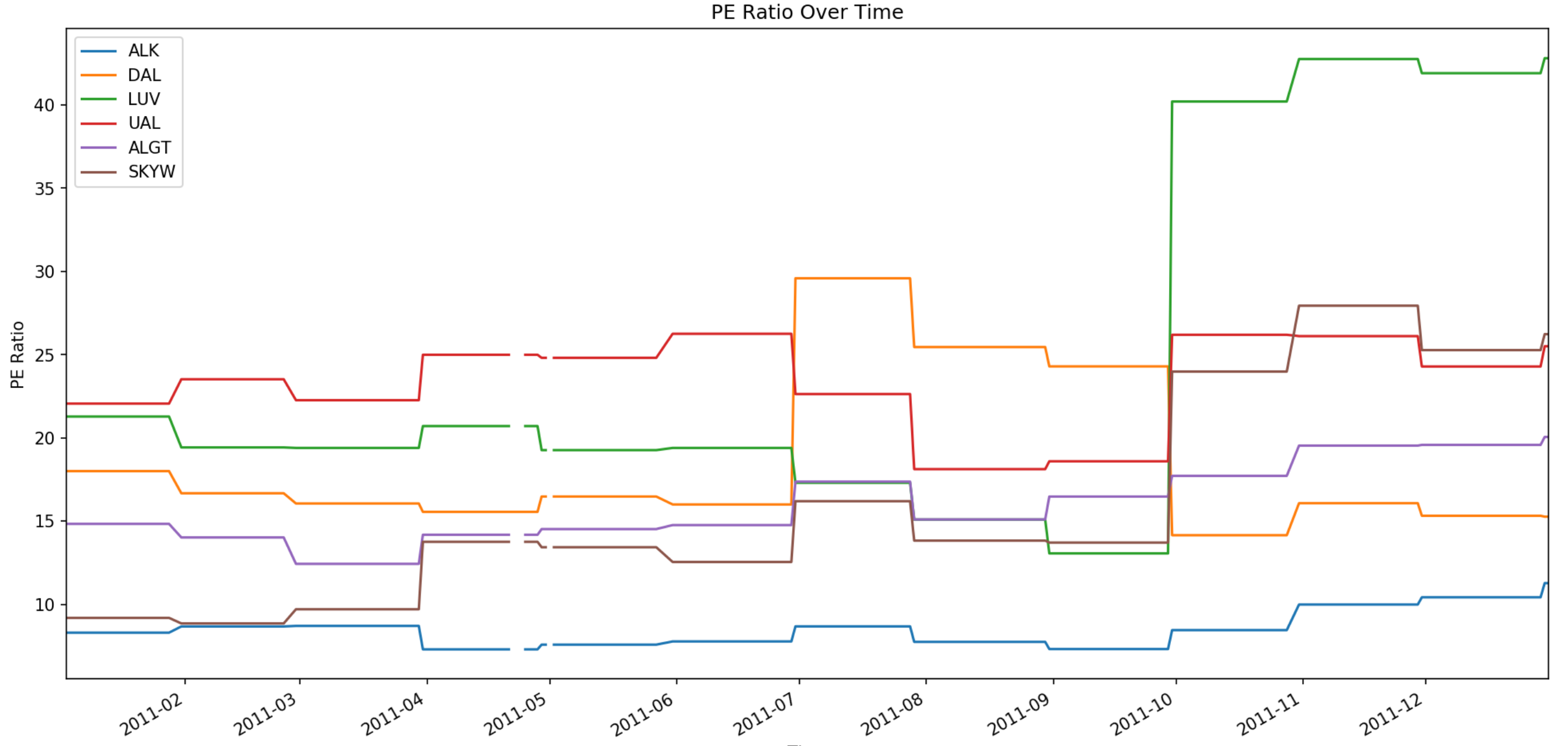
In order to see if lower PE ratio stocks do outperform higher PE ratio stocks, let's pick out the two airliners with the lowest and highest average PE Ratio over 2011.

# Sort stocks by their average PE ratio
sorted_by_mean_pe = pe_ratios.mean().sort_values()

We find that ALK had the lowest average PE ratio and LUV had the highest average PE ratio over 2011.. Let's plot their returns over the following years.

# Pick out stock with highest and lowest average PE ratio
highest_avg_pe = qb.Symbol(sorted_by_mean_pe.index[-1])
lowest_avg_pe = qb.Symbol(sorted_by_mean_pe.index[0])

# History request for 2012-2015 price data for our airlines
history = qb.History([highest_avg_pe, lowest_avg_pe], 
                     datetime(2012, 1, 1), 
                     datetime(2015, 1, 1), 
                     Resolution.Daily).close.unstack(level=0)

# Calculate daily cumulative returns
returns_over_time = ((history.pct_change()[1:] + 1).cumprod() - 1)

# Plot the return
returns_over_time.plot(figsize=(16, 8), title="Returns Over Time")
plt.ylabel("Return")
plt.show()