Optimizing a Gold-SPY Portfolio Using Hidden Markov Models for Market Downtime

This research focuses on constructing a dynamic portfolio combining a Gold ETF, GLD, and SPY to hedge against market downturns by utilizing Hidden Markov Models (HMM) for market regime detection as additional information. The strategy focuses on the downside risk by fitting an HMM with the SPY drawdown series. Then, we position size according to the probabilities for transitioning from the current regime to each candidate of the next regime, as the investor's views. The strategy yielded a Sharpe Ratio of 0.823 with a compounding annual return of 19.787% and a maximum drawdown of 27.1% over a 6-year backtest.

We used ETFs as vehicles since they are the most liquid. We chose GLD and SPY based on their complementary roles in a portfolio: GLD serves as a hedge during market downturns, while SPY represents the broader market. Their combination makes the portfolio more robust to withstand market drawdowns.

In finance, HMMs are often applied to detect market regimes by modeling hidden states representing different market conditions. Transition probabilities, which represent the likelihood of transitioning from the current state to all possible hidden states, are estimated to relate these states to the data so that HMMs can identify the most likely sequence of state transitions over time (Rabiner, 1989). The HMM input can also include significant exogenous variables to boost confidence when identifying a regime. In this study, hidden states were modeled by the drawdown series of SPY to determine if the current market is more likely to have greater or less drawdown. The drawdown series is defined as the peak-to-trough decline during a specific period.

Understanding the distribution of the drawdown series can allow us to pick the appropriate type of HMM to obtain a more accurate regime. Exploratory data analysis showed that the drawdown series was strongly and positively skewed (a heavy tail on the negative side). It reconciled with the Pickands-Balkema-de Haan theorem (Balkema & de Haan, 1974; Pickands, 1975), in which extreme values exceeding a threshold, like the drawdown series, can be approximated by a Generalized Pareto Distribution (GPD). Since it is not a Gaussian distribution, we need a Gaussian Mixture Model (GMM)-type HMM to model it. GMM is the mixture of multiple Gaussian distributions, which is useful for decomposing and approximating non-Gaussian distributions, including GPD (McLachlan & Peel, 2000). The following image shows the kernel distribution of the drawdown series and an example of its GMM decomposition. 

drawdown = history.rolling(20).apply(lambda a: (a.iloc[-1] - a.max()) / a.max()).dropna()
drawdown.plot(kind="kde", title="Kernel Distribution of SPY Drawdown", xlim=[-0.2, 0.05])

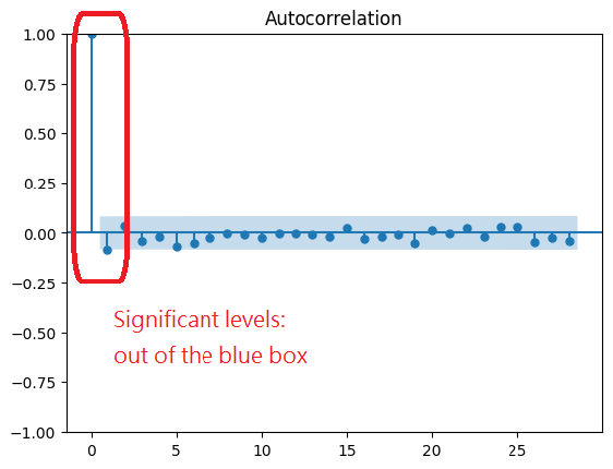
We also perform autocorrelation analysis to see if HMM can handle the drawdown series. The Autocorrelation Function (ACF) and Partial Autocorrelation Function (PACF) analyze the temporal dependencies in time series data. If any lag in ACF and PACF is significant, the previous regime provides information about the next regime, just like a Markov process. Hence, HMM is applicable. ACF measures the correlation between a series and its lagged versions, while PACF measures the correlation between the series and its lag but excludes the contributions from intermediate lags. We can observe that the drawdown series is highly autocorrelated with previous data points.

from statsmodels.graphics.tsaplots import plot_acf, plot_pacf
plot_acf(drawdown)
plot_pacf(drawdown)

In addition, since the ACF is declining slowly and the PACF has a damp sine wave decline, some information/variance has not been fully exploited. We again perform ACF and PACF analysis on the first differencing of the drawdown series to extract the information left out. The subsequent ACF and PACF showed 1-lag significance in the autocorrelation, hence we can incorporate the first differencing of the drawdown series as an exogenous variable to fit the HMM more accurately.

To implement this strategy, we start with the initialize method and request data for SPY and GLD.

self.spy = self.add_equity("SPY", Resolution.MINUTE).symbol
self.gold = self.add_equity("GLD", Resolution.MINUTE).symbol

We also add a Scheduled Event to rebalance the portfolio at the start of each week.

self.schedule.on(self.date_rules.week_start(self.spy), self.time_rules.after_market_open(self.spy, 1), self.rebalance)

The rebalance method fits a GMM HMM with the drawdown series of SPY to model the market drawdown regime.

def rebalance(self) -> None:
    history = self.history(self.spy, self.history_lookback*5, Resolution.DAILY).unstack(0).close.resample('W').last()
    drawdown = history.rolling(self.drawdown_lookback).apply(lambda a: (a.iloc[-1] - a.max()) / a.max()).dropna()
    inputs = np.concatenate([drawdown[[self.spy]].iloc[1:].values, drawdown[[self.spy]].diff().iloc[1:].values], axis=1)
    model = GMMHMM(n_components=2, n_mix=3, covariance_type='tied', n_iter=100, random_state=0).fit(inputs)

Then, the portfolio is rebalanced based on the transitional probabilities of the current state to the next possible states.

    self.set_holdings([PortfolioTarget(self.gold, next_prob_high),
                       PortfolioTarget(self.spy, 1 - next_prob_high)],
                      liquidate_existing_holdings=True)

The strategy was backtested in LEAN from 2019 to 2024. The benchmark is buy-and-hold SPY, which produced a 0.646 Sharpe Ratio.  The strategy yielded the following performance metrics over the backtest period.

We ran a parameter optimization job to test the sensitivity of the chosen parameters. We tested a historical data lookback window of 50 weeks to 150 weeks in steps of 25 weeks and a drawdown lookback window of 5 weeks to 40 weeks in steps of 5 weeks. Of the 40 parameter combinations, 11/40 (27.5%) produced a greater Sharpe ratio than the benchmark, and 40/40 (100.0%) made a smaller maximum drawdown than the benchmark.

The red circle in the preceding image identifies the parameters we chose as the strategy's default. We chose a historical data lookback window of 50 weeks and a drawdown lookback window of 20 weeks because they produced the best risk-adjusted return.

We further analyzed the strategy equity curve with SPY and GLD. Due to the risk diversification brought by the negative correlation between SPY and GLD, the strategy demonstrated robustness against the stock market shock in early 2020, the Gold market drop from late 2020 to 2021, and the 2022 market plummet. The strategy performed well compared to GLD and SPY in terms of return, volatility, and risk-adjusted return.

• Balkema, A. A., & de Haan, L. (1974). Residual life time at great age. The Annals of Probability, 2(5), 792-804.
• McLachlan, G. J., & Peel, D. (2000). Finite mixture models. John Wiley & Sons.
• Pickands, J. (1975). Statistical inference using extreme order statistics. The Annals of Statistics, 3(1), 119-131.
• Rabiner, L. R. (1989). A tutorial on hidden Markov models and selected applications in speech recognition. Proceedings of the IEEE, 77(2), 257-286.