Adjusted Trend on Futures

In the Fast Trend Following strategy, we used a trend filter to forecast the upcoming trend of Futures contracts and to determine position sizing. We also incorporated buffering to reduce trading fees. In this tutorial, we extend upon the previous strategy so that the size of the forecast is adjusted to reflect the probability that the trend reverses. This algorithm is a re-creation of strategy #12 from Advanced Futures Trading Strategies (Carver, 2023). The results show that adding more trend filters and adjusting the trend forecasts causes an increase in trading costs and a decrease in risk-adjusted returns.

The Fast Trend Following strategy used a single EMAC(16, 64) trend filter to produce forecasts. In this strategy, use the following trend filters:

• EMAC(2, 8)
• EMAC(4, 16)
• EMAC(8, 32)
• EMAC(16, 64)
• EMAC(32, 128)
• EMAC(64, 256)

The correlation from these trend filters is less than 1, so two individual filters from the set can confirm or negate the current trend direction. The fast EMA span of each EMAC follows a $2^n$ pattern and the slow EMA span of each EMAC is 4 times the length of the fast span. As Carver points out, “any ratio between the two moving average lengths of two and six gives statistically indistinguishable results” (p. 165).

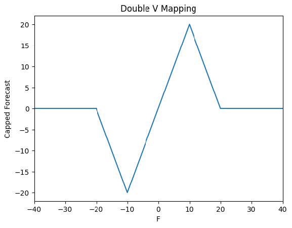
Carver analyzed the relationship between forecasts from the preceding EMAC trend filters and the realized risk adjusted returns following each forecast. He found that there is only a positive correlation between EMAC(2, 8) forecasts and risk adjusted returns when the forecasts are in the interval [-5, 5]. As a result, you should adjust the forecast capping of the EMAC(2, 8) trend filter from the previous strategy such that scaled forecasts ($F$) near zero are amplified and scaled forecasts further away from zero are dampened. Carver suggests the following “double V” mappings:

$$F < - 20: \textrm{Capped forecast} = 0$$ $$-20 < F < -10: \textrm{Capped forecast} = -40 - (2 \times F)$$ $$-10 < F < 10: \textrm{Capped forecast} = 2 \times F$$ $$10 < F < 20: \textrm{Capped forecast} = 40 - (2 \times F)$$ $$F > 20: \textrm{Capped forecast} = 0$$

The following image visualizes the “double V” mapping function:

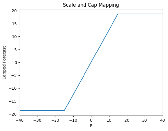
Carver also suggests adjusting the forecast capping of EMAC(4, 16) and EMAC(64, 256) to an absolute value of 15 instead of 20 and to apply a multiplier to ensure the forecasts still have the correct scaling. He suggests the following “scale and cap” mappings:

$$F < - 15: \textrm{Capped forecast} = -15 \times 1.25 = -18.75$$ $$-15 < F < 15: \textrm{Capped forecast} = F \times 1.25$$ $$F > 15: \textrm{Capped forecast} = 15 \times 1.25 = 18.75$$

The following image visualizes the “scale and cap” mapping function:

Let’s walk through how we can implement this trading algorithm with the LEAN trading engine. Most of the code is the same as the previous strategy, so the following sections only explain the differences with the Alpha model.

Initialization

In the Initialization method in main.py, we replace the Alpha model with a new one, the AdjustedTrendAlphaModel.

 from alpha import AdjustedTrendAlphaModel
class AdjustedTrendFuturesAlgorithm(QCAlgorithm):
    
    def Initialize(self):
        # . . .
        emac_filters = self.GetParameter("emac_filters", 6)
        blend_years = self.GetParameter("blend_years", 3)
        self.AddAlpha(AdjustedTrendAlphaModel(
            self,
            emac_filters, 
            self.GetParameter("abs_forecast_cap", 20),
            self.GetParameter("sigma_span", 32), 
            self.GetParameter("target_risk", 0.2),         
            blend_years
        ))

Alpha Model Constructor

We define the constructor of the Alpha model in the alpha.py file. The new constructor generates all of the EMA spans we need.

 from futures import categories
class AdjustedTrendAlphaModel(AlphaModel):
    BUSINESS_DAYS_IN_YEAR = 256
    def __init__(self, algorithm, emac_filters, abs_forecast_cap, sigma_span, target_risk, blend_years):
        self.algorithm = algorithm
        
        self.emac_spans = [2**x for x in range (1, self.emac_filters+1)]
        self.fast_ema_spans = self.emac_spans
        self.slow_ema_spans = [fast_span * 4 for fast_span in self.emac_spans] 
        self.all_ema_spans = sorted(list(set(self.fast_ema_spans + self.slow_ema_spans)))
        self.annulaization_factor = self.BUSINESS_DAYS_IN_YEAR ** 0.5
        self.abs_forecast_cap = abs_forecast_cap
        
        self.sigma_span = sigma_span
        self.target_risk = target_risk
        self.blend_years = blend_years
        self.idm = 1.5  # Instrument Diversification Multiplier
        self.categories = categories
        self.total_lookback = timedelta(365*self.blend_years+self.all_ema_spans[-1])
        self.day = -1
+ Expand
- Collapse

Creating Trend Filters

We adjust the OnSecuritiesChanged method in alpha.py to create the new EMAC trend filters we need.

 class AdjustedTrendAlphaModel(AlphaModel):
    def OnSecuritiesChanged(self, algorithm: QCAlgorithm, changes: SecurityChanges) -> None:
        for security in changes.AddedSecurities:
            symbol = security.Symbol
            # Create a consolidator to update the history
            security.consolidator = TradeBarConsolidator(timedelta(1))
            security.consolidator.DataConsolidated += self.consolidation_handler
            algorithm.SubscriptionManager.AddConsolidator(symbol, security.consolidator)
            if symbol.IsCanonical():
                # Add some members to track price history
                security.adjusted_history = pd.Series()
                security.raw_history = pd.Series()
                # Create indicators for the continuous contract
                ema_by_span = {span: algorithm.EMA(symbol, span, Resolution.Daily) for span in self.all_ema_spans}
                security.ewmac_by_span = {}
                for i, fast_span in enumerate(self.emac_spans):
                    security.ewmac_by_span[fast_span] = IndicatorExtensions.Minus(ema_by_span[fast_span], ema_by_span[self.slow_ema_spans[i]])
                security.automatic_indicators = ema_by_span.values()
                self.futures.append(security)
        for security in changes.RemovedSecurities:
            # Remove consolidator + indicators
            algorithm.SubscriptionManager.RemoveConsolidator(security.Symbol, security.consolidator)
            if security.Symbol.IsCanonical():
                for indicator in security.automatic_indicators:
                    algorithm.DeregisterIndicator(indicator)
+ Expand
- Collapse

Capping and Aggregating Forecasts

We adjust the Update method in alpha.py to apply the preceding forecast mappings and aggregate the forecasts from all the trend filters into a single value. To aggregate all the forecasts, use the following procedure:

1. Calculate the average of all the forecasts.
2. Multiply the result by a forecast diversification multiplier (FDM) to keep the average forecast at 10.
3. Cap the result to fall in the interval [-20, 20].

The FDM depends on the number of trend filters you use for the specific Future. If you determine some trend filters are too expensive to trade for the Future, you can remove their contributions to the final adjusted forecast. In this tutorial, we follow the example provided by Carter and use all of the trend filters.

 class AdjustedTrendAlphaModel(AlphaModel):
    FORECAST_SCALAR_BY_SPAN = {64: 1.91, 32: 2.79, 16: 4.1, 8: 5.95, 4: 8.53, 2: 12.1}        
    FDM_BY_RULE_COUNT = {1: 1.0, 2: 1.03, 3: 1.08, 4: 1.13, 5: 1.19, 6: 1.26}
    SCALE_AND_CAP_MAPPING_MULTIPLIER = 1.25
    def Update(self, algorithm: QCAlgorithm, data: Slice) -> List[Insight]:        
        # Record the new contract in the continuous series
        if data.QuoteBars.Count:
            for future in self.futures:
                future.latest_mapped = future.Mapped
        # If warming up and still > 7 days before start date, don't do anything
        # We use a 7-day buffer so that the algorithm has active insights when warm-up ends
        if algorithm.StartDate - algorithm.Time > timedelta(7):
            return []
        
        if self.day == data.Time.day or data.Bars.Count == 0:
            return []
        # Estimate the standard deviation of % daily returns for each future
        sigma_pct_by_future = {}
        for future in self.futures:
            # Estimate the standard deviation of % daily returns
            sigma_pct = self.estimate_std_of_pct_returns(future.raw_history, future.adjusted_history)
            if sigma_pct is None:
                continue
            sigma_pct_by_future[future] = sigma_pct
        
        # Create insights
        insights = []
        weight_by_symbol = GetPositionSize({future.Symbol: self.categories[future.Symbol] for future in sigma_pct_by_future.keys()})
        for symbol, instrument_weight in weight_by_symbol.items():
            future = algorithm.Securities[symbol]
            current_contract = algorithm.Securities[future.Mapped]
            daily_risk_price_terms = sigma_pct_by_future[future] / (self.annulaization_factor) * current_contract.Price # "The price should be for the expiry date we currently hold (not the back-adjusted price)" (p.55)
            # Calculate target position
            position = (algorithm.Portfolio.TotalPortfolioValue * self.idm * instrument_weight * self.target_risk) \
                      /(future.SymbolProperties.ContractMultiplier * daily_risk_price_terms * (self.annulaization_factor))
            # Adjust target position based on forecast
            capped_forecast_by_span = {}
            for span in self.emac_spans:
                risk_adjusted_ewmac = future.ewmac_by_span[span].Current.Value / daily_risk_price_terms
                scaled_forecast_for_ewmac = risk_adjusted_ewmac * self.FORECAST_SCALAR_BY_SPAN[span]
                
                if span == 2: # "Double V" forecast mapping (page 253-254)
                    if scaled_forecast_for_ewmac < -20:
                        capped_forecast_by_span[span] = 0
                    elif -20 <= scaled_forecast_for_ewmac < -10:
                        capped_forecast_by_span[span] = -40 - (2 * scaled_forecast_for_ewmac)
                    elif -10 <= scaled_forecast_for_ewmac < 10:
                        capped_forecast_by_span[span] = 2 * scaled_forecast_for_ewmac
                    elif 10 <= scaled_forecast_for_ewmac < 20:
                        capped_forecast_by_span[span] = 40 - (2 * scaled_forecast_for_ewmac)
                    else:
                        capped_forecast_by_span[span] = 0
                
                elif span in [4, 64]: # "Scale and cap" forecast mapping
                    if scaled_forecast_for_ewmac < -15:
                        capped_forecast_by_span[span] = -15 * self.SCALE_AND_CAP_MAPPING_MULTIPLIER
                    elif -15 <= scaled_forecast_for_ewmac < 15:
                        capped_forecast_by_span[span] = scaled_forecast_for_ewmac * self.SCALE_AND_CAP_MAPPING_MULTIPLIER
                    else:
                        capped_forecast_by_span[span] = 15 * self.SCALE_AND_CAP_MAPPING_MULTIPLIER
                
                else: # Normal forecast capping
                    capped_forecast_by_span[span] = max(min(scaled_forecast_for_ewmac, self.abs_forecast_cap), -self.abs_forecast_cap)
            
            raw_combined_forecast = sum(capped_forecast_by_span.values()) / len(capped_forecast_by_span) # Calculate a weighted average of capped forecasts (p. 194)
            scaled_combined_forecast = raw_combined_forecast * self.FDM_BY_RULE_COUNT[len(capped_forecast_by_span)] # Apply a forecast diversification multiplier to keep the average forecast at 10 (p 193-194)
            capped_combined_forecast = max(min(scaled_combined_forecast, self.abs_forecast_cap), -self.abs_forecast_cap)
            if capped_combined_forecast * position == 0:
                continue
            # Save some data for the PCM
            current_contract.forecast = capped_combined_forecast
            current_contract.position = position
            
            # Create the insights
            local_time = Extensions.ConvertTo(algorithm.Time, algorithm.TimeZone, future.Exchange.TimeZone)
            expiry = future.Exchange.Hours.GetNextMarketOpen(local_time, False) - timedelta(seconds=1)
            insights.append(Insight.Price(future.Mapped, expiry, InsightDirection.Up if capped_combined_forecast * position > 0 else InsightDirection.Down))
        
        if insights:
            self.day = data.Time.day
        return insights
+ Expand
- Collapse

We backtested the strategy from July 1, 2020 to July 1, 2023. The algorithm placed 909 trades, incurred $9,296.28 in fees, and achieved a 0.193 Sharpe ratio. In contrast, the Fast Trend Following strategy that uses a single EMAC trend filter and non-adjusted forecasts placed 607 trades, incurred $4,724.53 in fees, and achieved a 0.294 Sharpe ratio. Therefore, the addition of more trend filters and forecast adjustments causes the strategy to trade more frequently and reduces the risk-adjusted returns. 

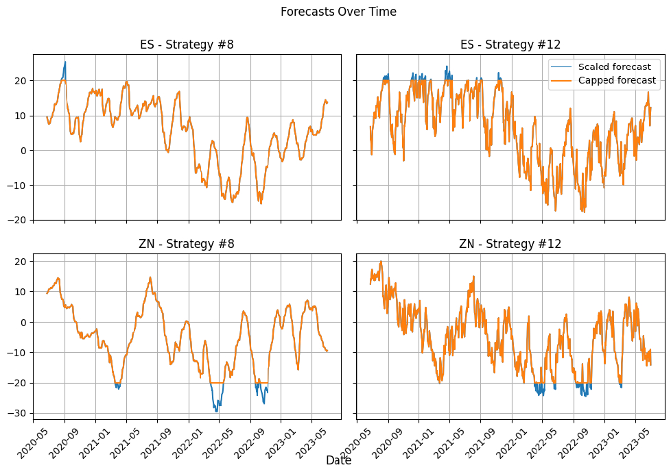
Trades and Fees Increase

We investigated why this strategy (#12) had more trades and fees than the Fast Trend Following strategy (#8). The following image shows the forecasts of both Futures for both strategies. The results show that the forecasts for strategy #12 have the same general shape as the forecasts for strategy #8, but the forecasts are more volatile in strategy #12. This increase in forecast volatility leads to an increase in trades and fees.

We used all of the EMAC trend filters explained above to produce the forecasts. However, as Carver outlines, it is beneficial to only incorporate trend filters that have a historical record of profitability after considering fees, turnover, and rolling costs. Since this strategy doesn’t remove any trend filters, it may incorporate unprofitable ones, leading to a decrease in risk-adjusted returns relative to strategy #8.

It’s not just the increase in commission fees that causes the Sharpe ratio to decrease relative to strategy #8. If we eliminate all commission fees from both strategies, strategy #8 achieves a 0.297 Sharpe ratio (see backtest) and strategy #12 achieves a 0.212 Sharpe ratio (see backtest).

Trade Buffer and Position Sizing

Finally, we tested whether the trade buffering and position sizing logic still improve the strategy’s risk-adjusted return. The results show that if we remove the trade buffering logic, the Sharpe ratio increases from 0.193 to 0.225 but the fees increase from $9,296.28 to $11,583.68 (see backtest). Furthermore, if we limit the position sizing to just 1, -1, or 0 contracts, the Sharpe ratio decreases to -0.071 (see backtest). Therefore, the position sizing logic is still essential to increasing the strategy’s risk-adjusted returns.

If you want to continue developing this strategy, some areas of further research include:

• Tracking the performance of each trend filter and remove the ones that are too expensive to trade
• Calculating FDM on the fly instead of using the hard-coded estimates provided above

1. Carver, R. (2023). Advanced Futures Trading Strategies: 30 fully tested strategies for multiple trading styles and time frames. Harriman House Ltd.