


Introduction
In this tutorial, we use a trend filter to forecast the upcoming trend of Futures contracts and to determine position sizing. We also add buffering to reduce trading fees. This algorithm is a re-creation of strategy #8 from Advanced Futures Trading Strategies (Carver, 2023). The results show that applying the trend filter and diversified position sizing logic to a portfolio of Futures contracts for the S&P 500 E-mini and 10-year treasury note outperforms a buy-and-hold benchmark strategy with the same contracts.
Forecasting Trends
A common technique to quantitatively classify the trend direction of an instrument is to use an exponential moving average crossover (EMAC) on historical prices.
\[\textrm{EMAC(16, 64)} = \textrm{EMA(16)} - \textrm{EMA(64)}\]
When the EMAC is positive, the instrument is in an uptrend and when the EMAC is negative, the instrument is in a downtrend. In the case of Futures, the EMA indicators are applied to the adjusted prices of the continuous contract because their adjusted prices remove price jumps that could give a false change of the EMAC sign.
The sign of the EMCA can only signal the trend direction for an individual security. To convert the EMAC value to something that you can use to compare the trend of two different securities, divide the EMAC value by the security’s standard deviation of returns.
\[\textrm{Raw forecast} = \frac{EMAC(16, 64)}{\sigma_p}\]
We want to know whether the raw forecast is relatively large or small for an individual security. To this end, we can divide the raw forecast by the average absolute value of trailing raw forecasts. Furthermore, Carver suggests scaling the forecast to have an average absolute value of 10 to make it easier to understand.
\[\textrm{Scaled forecast} = \textrm{Raw forecast} \times 10 \div \textrm{Average absolute value of raw forecast}\]
We can name the latter part of this equation the forecast scalar.
\[\textrm{Forecast scalar} = 10 \div \textrm{Average absolute value of raw forecast}\]
\[\textrm{Scaled forecast} = \textrm{Raw forecast} \times \textrm{Forecast scalar}\]
Carver provides the forecast scalar value of 4.1 for this strategy.
\[\textrm{Scaled forecast} = \textrm{Raw forecast} \times 4.1\]
We then cap the scaled forecast to fall within the interval [-20, 20].
\[\textrm{Capped forecast} = \max(\min(\textrm{Scaled forecast}, 20), -20)\]
The capped forecast is a factor used to determine our Future contract trade direction and position size.
Position Sizing
To determine the optimal position size of each Future under consideration, we use the following formula:
\[N_{i,t} = \frac{\textrm{Capped forecast}_{i,t} \times \textrm{Capital} \times \textrm{IDM} \times \textrm{Weight}_i \times \tau }{10 \times \textrm{Multiplier}_i \times \textrm{Price}_{i,t} \times \sigma_{\%i,t}}\]
where
- \(N_{i,t}\) is the number of contracts to hold for instrument \(i\) at time \(t\).
- \(\textrm{Capped forecast}_{i,t}\) is the capped forecast of instrument \(i\) at time \(t\).
- \(\textrm{Capital}\) is the current total portfolio value.
- \(\textrm{IDM}\) is the instrument diversification multiplier. Carver provides a methodology for dynamically calculating the IDM in later strategies, but this algorithm only trades two instruments, so we follow the recommendation of setting the IDM to 1.5.
- \(\textrm{Weight}_i\) is the classification weight of instrument \(i\). The algorithm we create here only trades 2 Futures, so \(\textrm{Weight}_i\) always 0.5.
- \(\tau\) is the target portfolio risk. This is oftentimes a subjective value that’s a function of the investor’s risk profile. In this algorithm, we use the recommended value of 0.2 (20%) from Carver.
- \(\textrm{Multiplier}_i\) is the contract multiplier of instrument \(i\).
- \(\textrm{Price}_{i,t}\) is the price of instrument \(i\) at time \(t\).
- \(\sigma_{\%i,t}\) is the annualized risk of instrument \(i\) at time \(t\).
Trading Buffers
To avoid very small orders and reduce trading fees, we set a trading buffer. The trading buffer is a region surrounding the optimal position size where we don’t bother trading. To calculate the buffer size, we apply a fraction \(F\) in the following equation:
\[B_{i,t} = \frac{\textrm{F} \times \textrm{Capital} \times \textrm{IDM} \times \textrm{Weight}_i \times \tau }{\textrm{Multiplier}_i \times \textrm{Price}_{i,t} \times \sigma_{\%i,t}}\]
It’s possible to calculate \(F\) from factors like the profitability of the trading rule and its associated costs, but Carver suggests a conservative value of 0.1 (10%).
Next, we can calculate the lower and upper boundaries of the buffer.
\[B^U_{i,t} = round(N_{i,t} + B_{i,t})\]
\[B^L_{i,t} = round(N_{i,t} - B_{i,t})\]
Therefore, if our current holdings are above the buffer, we rebalance to be at \(B^U_{i,t}\). If our current holdings are below the buffer, we rebalance to be at \(B^L_{i,t}\). If our current holdings are inside the buffer zone, we don’t adjust the position.
Method
Let’s walk through how we can implement this trading algorithm with the LEAN trading engine.
Initialization
We start with the Initialization method, where we set the start date, end date, cash, and some settings.
class FuturesFastTrendFollowingLongAndShortWithTrendStrenthAlgorithm(QCAlgorithm):def initialize(self):self.set_start_date(2020, 7, 1)self.set_end_date(2023, 7, 1)self.set_cash(1_000_000)self.set_brokerage_model(BrokerageName.INTERACTIVE_BROKERS_BROKERAGE, AccountType.MARGIN)self.set_security_initializer(BrokerageModelSecurityInitializer(self.brokerage_model, FuncSecuritySeeder(self.get_last_known_prices)))self.settings.minimum_order_margin_portfolio_percentage = 0
Universe Selection
We follow the example algorithm outlined in the book and configure the Universe Selection model to return Futures contracts for the S&P 500 E-mini and 10-year treasury note. To accomplish this, follow these steps:
1. In the futures.py file, define the Futures symbols and their respective market category.
categories = {Symbol.create(Futures.financials.y10_treasury_note, SecurityType.FUTURE, Market.CBOT): ("Fixed Income", "Bonds"),Symbol.create(Futures.indices.SP500E_MINI, SecurityType.FUTURE, Market.CME): ("Equity", "US")}
2. In the universe.py file, import the categories and define the Universe Selection model.
from Selection.FutureUniverseSelectionModel import FutureUniverseSelectionModelfrom futures import categoriesclass AdvancedFuturesUniverseSelectionModel(FutureUniverseSelectionModel):def __init__(self) -> None:super().__init__(timedelta(1), self.select_future_chain_symbols)self.symbols = list(categories.keys())def select_future_chain_symbols(self, utc_time: datetime) -> List[Symbol]:return self.symbolsdef filter(self, filter: FutureFilterUniverse) -> FutureFilterUniverse:return filter.expiration(0, 365)
3. In the main.py file, extend the Initialization method to configure the universe settings and add a Universe Selection model.
class FuturesFastTrendFollowingLongAndShortWithTrendStrenthAlgorithm(QCAlgorithm):def initialize(self):# . . .self.universe_settings.data_normalization_mode = DataNormalizationMode.BACKWARDS_PANAMA_CANALself.universe_settings.data_mapping_mode = DataMappingMode.OPEN_INTERESTself.add_universe_selection(AdvancedFuturesUniverseSelectionModel())
To form the continuous contract price series, select the current contract based on open interest and adjust historical prices using the BackwardsPanamaCanal DataNormalizationMode. Note that the original algorithm by Carver rolls over contracts \(n\) days before they expire instead of rolling based on open interest, so our results will be slightly different.
Forecasting Future Trends
We first define the constructor of the Alpha model in the alpha.py file.
+ Expand
from futures import categoriesclass FastTrendFollowingLongAndShortWithTrendStrenthAlphaModel(AlphaModel):BUSINESS_DAYS_IN_YEAR = 256FORECAST_SCALAR_BY_SPAN = {64: 1.91, 32: 2.79, 16: 4.1, 8: 5.95, 4: 8.53, 2: 12.1}def __init__(self, algorithm, slow_ema_span, abs_forecast_cap, sigma_span, target_risk, blend_years):self.algorithm = algorithmself.slow_ema_span = slow_ema_spanself.slow_ema_smoothing_factor = self.calculate_smoothing_factor(self.slow_ema_span)self.fast_ema_span = int(self.slow_ema_span / 4)self.fast_ema_smoothing_factor = self.calculate_smoothing_factor(self.fast_ema_span)self.annulaization_factor = self.BUSINESS_DAYS_IN_YEAR ** 0.5self.abs_forecast_cap = abs_forecast_capself.sigma_span = sigma_spanself.target_risk = target_riskself.blend_years = blend_yearsself.idm = 1.5self.forecast_scalar = self.FORECAST_SCALAR_BY_SPAN[self.fast_ema_span]self.categories = categoriesself.total_lookback = timedelta(365*self.blend_years+self.slow_ema_span)self.day = -1
When new Futures are added to the universe, we set up a consolidator to keep the trailing data updated as the algorithm executes. If the security that’s added is a continuous contract, we combine two EMA indicators to create the EMAC.
+ Expand
class FastTrendFollowingLongAndShortWithTrendStrenthAlphaModel(AlphaModel):def on_securities_changed(self, algorithm: QCAlgorithm, changes: SecurityChanges) -> None:for security in changes.added_securities:symbol = security.symbol# Create a consolidator to update the historysecurity.consolidator = TradeBarConsolidator(timedelta(1))security.consolidator.data_consolidated += self.consolidation_handleralgorithm.subscription_manager.add_consolidator(symbol, security.consolidator)if security.symbol.is_canonical():# Add some members to track price historysecurity.adjusted_history = pd.Series()security.raw_history = pd.Series()# Create indicators for the continuous contractsecurity.fast_ema = algorithm.EMA(security.symbol, self.fast_ema_span, Resolution.DAILY)security.slow_ema = algorithm.EMA(security.symbol, self.slow_ema_span, Resolution.DAILY)security.ewmac = IndicatorExtensions.minus(security.fast_ema, security.slow_ema)security.automatic_indicators = [security.fast_ema, security.slow_ema]self.futures.append(security)for security in changes.removed_securities:# Remove consolidator + indicatorsalgorithm.subscription_manager.remove_consolidator(security.symbol, security.consolidator)if security.symbol.is_canonical():for indicator in security.automatic_indicators:algorithm.deregister_indicator(indicator)
The consolidation handler simply updates the security history and trims off any history that’s too old.
class FastTrendFollowingLongAndShortWithTrendStrenthAlphaModel(AlphaModel):def consolidation_handler(self, sender: object, consolidated_bar: TradeBar) -> None:security = self.algorithm.securities[consolidated_bar.symbol]end_date = consolidated_bar.end_time.date()if security.symbol.is_canonical():# Update adjusted historysecurity.adjusted_history.loc[end_date] = consolidated_bar.closesecurity.adjusted_history = security.adjusted_history[security.adjusted_history.index >= end_date - self.total_lookback]else:# Update raw historycontinuous_contract = self.algorithm.securities[security.symbol.canonical]if consolidated_bar.symbol == continuous_contract.latest_mapped:continuous_contract.raw_history.loc[end_date] = consolidated_bar.closecontinuous_contract.raw_history = continuous_contract.raw_history[continuous_contract.raw_history.index >= end_date - self.total_lookback]
Next, we define a helper method to estimate the standard deviation of returns.
+ Expand
class FastTrendFollowingLongAndShortWithTrendStrenthAlphaModel(AlphaModel):def estimate_std_of_pct_returns(self, raw_history, adjusted_history):# Align history of raw and adjusted pricesidx = sorted(list(set(adjusted_history.index).intersection(set(raw_history.index))))adjusted_history_aligned = adjusted_history.loc[idx]raw_history_aligned = raw_history.loc[idx]# Calculate exponentially weighted standard deviation of returnsreturns = adjusted_history_aligned.diff().dropna() / raw_history_aligned.shift(1).dropna()rolling_ewmstd_pct_returns = returns.ewm(span=self.sigma_span, min_periods=self.sigma_span).std().dropna()if rolling_ewmstd_pct_returns.empty: # Not enough historyreturn None# Annualize sigma estimateannulized_rolling_ewmstd_pct_returns = rolling_ewmstd_pct_returns * (self.annulaization_factor)# Blend the sigma estimate (p.80)blended_estimate = 0.3*annulized_rolling_ewmstd_pct_returns.mean() + 0.7*annulized_rolling_ewmstd_pct_returns.iloc[-1]return blended_estimate
The Update method calculates the forecast of the Futures at the beginning of each trading day and returns some Insight objects for the Portfolio Construction model.
+ Expand
class FastTrendFollowingLongAndShortWithTrendStrenthAlphaModel(AlphaModel):def update(self, algorithm: QCAlgorithm, data: Slice) -> List[Insight]:# Record the new contract in the continuous seriesif data.quote_bars.count:for future in self.futures:future.latest_mapped = future.mapped# If warming up and still > 7 days before start date, don't do anything# We use a 7-day buffer so that the algorithm has active insights when warm-up endsif algorithm.start_date - algorithm.time > timedelta(7):return []if self.day == data.time.day or data.bars.count == 0:return []# Estimate the standard deviation of % daily returns for each futuresigma_pct_by_future = {}for future in self.futures:# Estimate the standard deviation of % daily returnssigma_pct = self.estimate_std_of_pct_returns(future.raw_history, future.adjusted_history, future)if sigma_pct is None:continuesigma_pct_by_future[future] = sigma_pct# Create insightsinsights = []weight_by_symbol = GetPositionSize({future.symbol: self.categories[future.symbol] for future in sigma_pct_by_future.keys()})for symbol, instrument_weight in weight_by_symbol.items():future = algorithm.securities[symbol]current_contract = algorithm.securities[future.mapped]daily_risk_price_terms = sigma_pct_by_future[future] / (self.annulaization_factor) * current_contract.price # "The price should be for the expiry date we currently hold (not the back-adjusted price)" (p.55)# Calculate target positionposition = (algorithm.portfolio.total_portfolio_value * self.idm * instrument_weight * self.target_risk) \/(future.symbol_properties.contract_multiplier * daily_risk_price_terms * (self.annulaization_factor))# Adjust target position based on forecastrisk_adjusted_ewmac = future.ewmac.current.value / daily_risk_price_termsscaled_forecast_for_ewmac = risk_adjusted_ewmac * self.forecast_scalarforecast = max(min(scaled_forecast_for_ewmac, self.abs_forecast_cap), -self.abs_forecast_cap)if forecast * position == 0:continue# Save some data for the PCMcurrent_contract.forecast = forecastcurrent_contract.position = position# Create the insightslocal_time = Extensions.convert_to(algorithm.time, algorithm.time_zone, future.exchange.time_zone)expiry = future.exchange.hours.get_next_market_open(local_time, False) - timedelta(seconds=1)insights.append(Insight.price(future.mapped, expiry, InsightDirection.UP if forecast * position > 0 else InsightDirection.DOWN))if insights:self.day = data.time.dayreturn insights
Finally, to add the Alpha model to the algorithm, we extend the Initialization method in the main.py file to set the new Alpha model and add a warm-up period.
+ Expand
from alpha import FastTrendFollowingLongAndShortWithTrendStrenthAlphaModelclass FuturesFastTrendFollowingLongAndShortWithTrendStrenthAlgorithm(QCAlgorithm):def initialize(self):# . . .slow_ema_span = 2 ** self.get_parameter("slow_ema_span_exponent", 6)blend_years = self.get_parameter("blend_years", 3)self.add_alpha(FastTrendFollowingLongAndShortWithTrendStrenthAlphaModel(self,slow_ema_span,self.get_parameter("abs_forecast_cap", 20),self.get_parameter("sigma_span", 32),self.get_parameter("target_risk", 0.2),blend_years))self.set_warm_up(timedelta(365*blend_years + slow_ema_span + 7))
Calculating Position Sizes
We first define a custom Portfolio Construction model in the portfolio.py file that calculates the optimal position for each Future and applies the buffer zone logic.
+ Expand
class BufferedPortfolioConstructionModel(EqualWeightingPortfolioConstructionModel):def __init__(self, rebalance, buffer_scaler):super().__init__(rebalance)self.buffer_scaler = buffer_scalerdef create_targets(self, algorithm: QCAlgorithm, insights: List[Insight]) -> List[PortfolioTarget]:targets = super().create_targets(algorithm, insights)adj_targets = []for insight in insights:future_contract = algorithm.securities[insight.symbol]optimal_position = future_contract.forecast * future_contract.position / 10# Create buffer zone to reduce churnbuffer_width = self.buffer_scaler * abs(future_contract.position)upper_buffer = round(optimal_position + buffer_width)lower_buffer = round(optimal_position - buffer_width)# Determine quantity to put holdings into buffer zonecurrent_holdings = future_contract.holdings.quantityif lower_buffer <= current_holdings <= upper_buffer:continuequantity = lower_buffer if current_holdings < lower_buffer else upper_buffer# Place tradesadj_targets.append(PortfolioTarget(insight.symbol, quantity))# Liquidate contracts that have an expired insightfor target in targets:if target.quantity == 0:adj_targets.append(target)return adj_targets
Then to add the Portfolio Construction model to the algorithm, we extend the Initialization method in the main.py file to set the new model.
+ Expand
from portfolio import BufferedPortfolioConstructionModelclass FuturesFastTrendFollowingLongAndShortWithTrendStrenthAlgorithm(QCAlgorithm):def initialize(self):# . . .self.settings.rebalance_portfolio_on_security_changes = Falseself.settings.rebalance_portfolio_on_insight_changes = Falseself.total_count = 0self.day = -1self.set_portfolio_construction(BufferedPortfolioConstructionModel(self.rebalance_func,self.get_parameter("buffer_scaler", 0.1) # Hardcoded on p.167 & p.173))def rebalance_func(self, time):if (self.total_count != self.insights.total_count or self.day != self.time.day) and not self.is_warming_up and self.current_slice.quote_bars.count > 0:self.total_count = self.insights.total_countself.day = self.time.dayreturn timereturn None
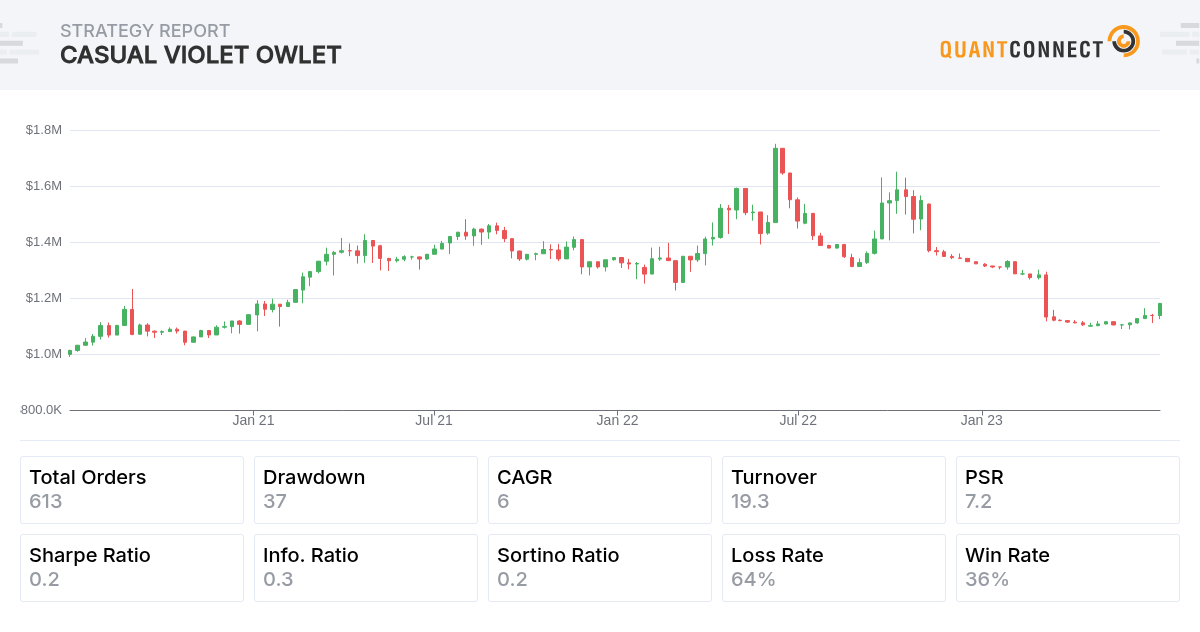
Results
We backtested the strategy from July 1, 2020 to July 1, 2023. The algorithm placed 607 trades, incurred $4,724.53 in fees, and achieved a 0.294 Sharpe ratio. In contrast, if we remove the trade buffering logic, the algorithm places 738 trades, incurs $5,607.51 in fees, and achieves a 0.301 Sharpe ratio (see backtest). Therefore, the buffering logic decreased the trades and fees, but also slightly decreased the Sharpe ratio.
A second benchmark to compare the strategy to is a buy-and-hold portfolio with variable risk position sizing applied to the same Futures contracts. This benchmark achieves a -0.335 Sharpe ratio (see backtest), so the strategy outperforms it in terms of risk-adjusted returns.
Lastly, we found the position sizing logic is vital to the success of the strategy. The backtest shows that the exposure ranges from -1,000% to 1,000%. However, if we cap \(N_{i,t}\) to fall in the interval [-1, 1], then the Sharpe ratio drops from 0.294 to 0.129 (see backtest).
Further Research
If you want to continue developing this strategy, some areas of further research include:
- Increasing the universe size
- Adjusting parameter values
- Incorporating the estimate of IDM
- Adjusting the rollover timing to match the timing outlined by Carver
References
- Carver, R. (2023). Advanced Futures Trading Strategies: 30 fully tested strategies for multiple trading styles and time frames. Harriman House Ltd.


Eko1900
The algorithm returns an error as below:
Runtime Error: 'datetime.timedelta' object has no attribute 'data_consolidated'
at OnSecuritiesChanged
security.consolidator.data_consolidated += self.consolidation_handler
^^^^^^^^^^^^^^^^^^^^^^^^^^^^^^^^^^^^^^^
in alpha.py: line 123
The material on this website is provided for informational purposes only and does not constitute an offer to sell, a solicitation to buy, or a recommendation or endorsement for any security or strategy, nor does it constitute an offer to provide investment advisory services by QuantConnect. In addition, the material offers no opinion with respect to the suitability of any security or specific investment. QuantConnect makes no guarantees as to the accuracy or completeness of the views expressed in the website. The views are subject to change, and may have become unreliable for various reasons, including changes in market conditions or economic circumstances. All investments involve risk, including loss of principal. You should consult with an investment professional before making any investment decisions.
Brandon Goyette
Looking to try “Increasing the universe size” - but unable to get it to work, and I've been unable to find similar examples to mimic.
i.e. lets add CL to the mix
categories = {
Symbol.create(Futures.Energy.CRUDE_OIL_WTI, Market.NYMEX): ("Energy", "Oil"),
Symbol.create(Futures.Financials.Y_10_TREASURY_NOTE, SecurityType.FUTURE, Market.CBOT): ("Fixed Income", "Bonds"),
Symbol.create(Futures.Indices.SP_500_E_MINI, SecurityType.FUTURE, Market.CME): ("Equity", "US")
}
The material on this website is provided for informational purposes only and does not constitute an offer to sell, a solicitation to buy, or a recommendation or endorsement for any security or strategy, nor does it constitute an offer to provide investment advisory services by QuantConnect. In addition, the material offers no opinion with respect to the suitability of any security or specific investment. QuantConnect makes no guarantees as to the accuracy or completeness of the views expressed in the website. The views are subject to change, and may have become unreliable for various reasons, including changes in market conditions or economic circumstances. All investments involve risk, including loss of principal. You should consult with an investment professional before making any investment decisions.
To unlock posting to the community forums please complete at least 30% of Boot Camp.
You can continue your Boot Camp training progress from the terminal. We hope to see you in the community soon!