Head & Shoulders TA Pattern Detection

Introduction

Technical analysis traders usually use graphical patterns to identify trading opportunities. Quant traders don't typically utilize these patterns in their automated trading systems because their presence is subjective, and they’re challenging to accurately detect. As a result, if these patterns have predictive power on future price movements, quant traders are missing an opportunity. To put it to the test, this tutorial explains a method to programmatically detect a popular graphical pattern in an event-driven trading algorithm. The results show that with just a simple time-based exit, the algorithm achieves greater risk-adjusted returns than the underlying benchmarks over the backtesting period.

Pattern Description

The pattern we use in this algorithm is the head and shoulders pattern, but this research can be extended to other graphical patterns. The head and shoulders pattern is characterized by two shoulders, a neckline, and a tall head in the middle.

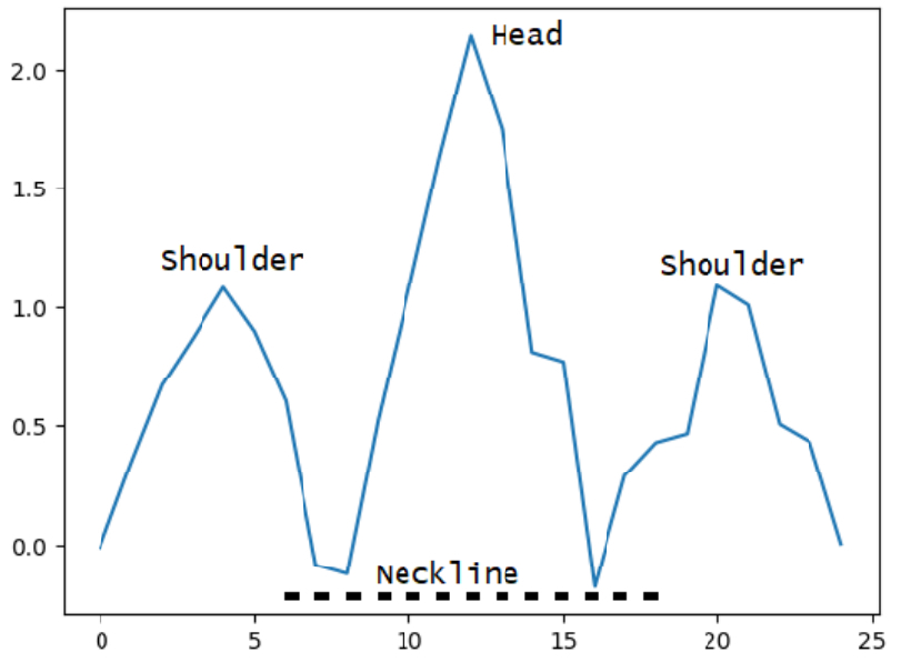
Some technical traders claim that the head and shoulders pattern signals an upcoming bullish-to-bearish trend reversal and that the neckline acts as a level of support.

Method

Let’s walk through how we can implement a head and shoulders trading algorithm with the LEAN trading engine.

Initialization

During initialization, we define some class variables, load all the algorithm parameters, and then add a coarse universe.

class HeadAndShouldersPatternDetectionAlgorithm(QCAlgorithm):
   trades = []
   new_symbols = []
   pattern_by_symbol = {}
   
   def initialize(self):
       self.set_start_date(2022, 1, 1)
       self.set_end_date(2023, 6, 1)
       self.set_cash(100000)
       
       # Pattern detection settings
       self.window_size = self.get_parameter("window_size", 25)
       self.max_lookback = self.get_parameter("max_lookback", 50)
       self.step_size = self.get_parameter("step_size", 10) 
       
       # Universe settings
       self.coarse_size = self.get_parameter("coarse_size", 500)
       self.universe_size = self.get_parameter("universe_size", 5)
       
       # Trade settings
       self.hold_duration = timedelta(self.get_parameter("hold_duration", 3))
       
       # Define universe
       self.universe_settings.resolution = Resolution.DAILY
       self.add_universe(self.coarse_filter_function)

Creating Pattern Detection Objects

We want to detect the presence of the head and shoulders pattern for as many securities as possible, so we scan for it once a day during universe selection. To ensure that we stay within the 10-minute quota for each step in the algorithm, we first reduce the number of coarse objects to only include the top 500 most liquid US Equities. Then, to enable us to scan for the pattern, we create HeadAndShouldersPattern objects for each US Equity in the subset of coarse objects.

def coarse_filter_function(self, coarse: List[CoarseFundamental]) -> List[Symbol]:
   coarse = sorted(coarse, key=lambda x: x.dollar_volume, reverse=True)[:self.coarse_size]
   
   # Create pattern detection objects for new securities
   coarse_symbols = [c.symbol for c in coarse]
   new_symbols = [symbol for symbol in coarse_symbols if symbol not in self.pattern_by_symbol]
   if new_symbols:
       history = self.history(new_symbols, self.max_lookback, Resolution.DAILY)
       for symbol in new_symbols:
           self.pattern_by_symbol[symbol] = HeadAndShouldersPattern(
               history.loc[symbol]['close'].values if symbol in history.index else np.array([]), 
               self.window_size, 
               self.max_lookback, 
               self.step_size
           )
           
   # Remove pattern detection objects for delisted securities
   delisted_symbols = [symbol for symbol in self.pattern_by_symbol.keys() if symbol not in coarse_symbols]
   for symbol in delisted_symbols:
       self.pattern_by_symbol.pop(symbol)
   # . . .

Generating Reference Patterns

To determine when the pattern occurs, we need to first generate many instances of the pattern. We need many unique samples to avoid a single, idealized pattern, so we add an element of randomness to each reference pattern. The following plot visualizes the data we generated:

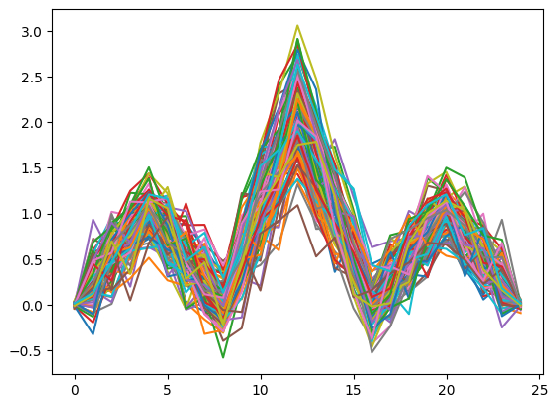
We generate this data during the construction of the first HeadAndShouldersPattern object and save it in a DataFrame as a static variable. The end of the constructor also scans the historical data sequence that we pass to the constructor to warm-up the detection system.

class HeadAndShouldersPattern(TechnicalPattern):
   def __init__(self, sequence, window_size, max_lookback, step_size):
       self.sequence = sequence
       self.window_size = window_size
       self.max_lookback = max_lookback
       self.step_size = step_size
       
       # Create pattern references
       if not hasattr(HeadAndShouldersPattern, "ref"):
           np.random.seed(1)
           ref_count = 100
           v1 = np.array([0] * ref_count) + 0.02 * norm.rvs(size=(ref_count, ))
           p1 = np.array([1] * ref_count) + 0.2 * norm.rvs(size=(ref_count, ))
           v2 = v1 + 0.2 * norm.rvs(size=(ref_count, ))
           v3 = v1 + 0.2 * norm.rvs(size=(ref_count, ))
           p3 = p1 + 0.02 * norm.rvs(size=(ref_count, ))
           p2 = 1.5 * np.maximum(p1, p3) + abs(uniform.rvs(size=(ref_count, )))
           v4 = v1 + 0.02 * norm.rvs(size=(ref_count, ))
           ref = pd.DataFrame([
               v1, 
               (v1*.75+p1*.25) + 0.2 * norm.rvs(size=(ref_count, )), 
               (v1+p1)/2 + 0.2 * norm.rvs(size=(ref_count, )), 
               (v1*.25+p1*.75) + 0.2 * norm.rvs(size=(ref_count, )), 
               p1, 
               (v2*.25+p1*.75) + 0.2 * norm.rvs(size=(ref_count, )), 
               (v2+p1)/2 + 0.2 * norm.rvs(size=(ref_count, )), 
               (v2*.75+p1*.25) + 0.2 * norm.rvs(size=(ref_count, )), 
               v2, 
               (v2*.75+p2*.25) + 0.2 * norm.rvs(size=(ref_count, )), 
               (v2+p2)/2 + 0.2 * norm.rvs(size=(ref_count, )), 
               (v2*.25+p2*.75) + 0.2 * norm.rvs(size=(ref_count, )), 
               p2, 
               (v3*.25+p2*.75) + 0.2 * norm.rvs(size=(ref_count, )), 
               (v3+p2)/2 + 0.2 * norm.rvs(size=(ref_count, )), 
               (v3*.75+p2*.25) + 0.2 * norm.rvs(size=(ref_count, )), 
               v3, 
               (v3*.75+p3*.25) + 0.2 * norm.rvs(size=(ref_count, )), 
               (v3+p3)/2 + 0.2 * norm.rvs(size=(ref_count, )), 
               (v3*.25+p3*.75) + 0.2 * norm.rvs(size=(ref_count, )), 
               p3, 
               (v4*.25+p3*.75) + 0.2 * norm.rvs(size=(ref_count, )), 
               (v4+p3)/2 + 0.2 * norm.rvs(size=(ref_count, )), 
               (v4*.75+p3*.25) + 0.2 * norm.rvs(size=(ref_count, )), 
               v4
           ])
           HeadAndShouldersPattern.ref = ((ref - ref.mean()) / ref.std()).T
           
       # Warm up the factor values
       self.rows = HeadAndShouldersPattern.ref.shape[0]
       self.scan()

Quantifying the Pattern Presence

After we create new HeadAndShouldersPattern objects for the new securities in the universe selection function, we update each object with their most recent price data.

def coarse_filter_function(self, coarse: List[CoarseFundamental]) -> List[Symbol]:
   # . . .
   for c in coarse:
       if c.symbol not in new_symbols:
           self.pattern_by_symbol[c.symbol].update(c.adjusted_price)
   # . . .

This update method updates the historical data in the HeadAndShouldersPattern objects and scans for patterns in the new data.

def update(self, price):
   self.sequence = np.append(self.sequence, price)[-self.max_lookback:]
   self.scan()

The scan method is where we quantify the presence of the pattern. This method calculates two factors for every security in the universe: correlation and Distance Time Warp (DTW) distance when compared to the reference patterns. It calculates these factors through the following procedure:

1. Select lookback windows of varying lengths.
2. Down-sample the lookback window to the same number of data points in the reference patterns, keeping the general shape but reducing the number of data points. 
3. Normalize the data in the trailing window.
4. Calculate the correlation and DTW distance between the data in the trailing window and the data in each reference pattern. 
5. To aggregate the results into 2 factor values, take the max of the current factor value and the mean of the factor values across the reference patterns.

def scan(self):
   self.corr = 0
   self.similarity_score = 0
   
   # Select varying lengths of trailing windows
   for i in range(self.window_size, self.max_lookback, self.step_size):
       # Check if enough history to fill the trailing window
       if len(self.sequence[-i:]) != i:
           break
           
       # Select the trailing data and downsample it to 25 data points
       #  to match the number of data points in each reference pattern.
       # Downsampling allows us to detect the pattern across varying time scales, 
       #  large patterns and small patterns.
       sub_sequence = np.array(self.downsample(self.sequence[-i:], self.window_size))
       
       # Normalize the data in the trailing window
       if sub_sequence.std() == 0:
           continue
       norm_sub_sequence = (sub_sequence - sub_sequence.mean()) / sub_sequence.std()
       
       # Evaluate the pattern presence
       # Calculate correlation and similarity scores for each reference pattern
       corr_scores = np.ndarray(shape=(self.rows))
       similarity_scores = np.ndarray(shape=(self.rows))
       for j in range(self.rows):
           score, similarity = self.matching(norm_sub_sequence, self.ref.iloc[j, :])
           corr_scores[j] = score
           similarity_scores[j] = similarity
           
       # After reviewing all of the reference patterns across varying lengths of lookback windows,
       # aggregate the results to produce a single value for each factor (correlation and similarity)
       self.corr = max(self.corr, corr_scores.mean())
       self.similarity_score = max(self.similarity_score, similarity_scores.mean())

The matching method applies a Savitzky-Golay filter to smooth the data in the lookback window and then calculates the DTW distance and correlation coefficient between the lookback window and the reference pattern.

class TechnicalPattern:
   def matching(self, series: np.array, ref: np.array) -> np.array:
       series_ = savgol_filter(series, 3, 2)
       series_ = (series_ - series_.mean()) / series_.std()
       path, similarity = dtw_path(ref, series_)
       series_ = np.array([series_[x[1]] for x in path])
       ref = np.array([ref[x[0]] for x in path])
       score = np.corrcoef(series_, ref)[0, 1]
       return score, similarity

To view the definition of the downsample method, see the technical_pattern.py file in the attached project.

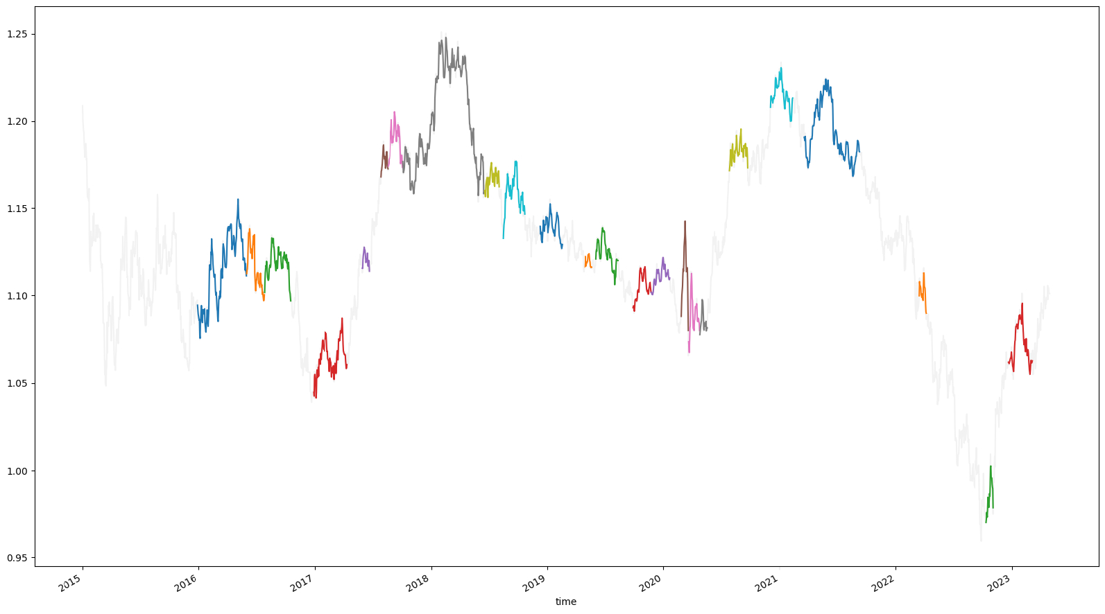
The following image shows regions in a price series with high correlation and low DTW distance, which lead to a stronger head and shoulders signal. Note the varying sizes of the highlighted regions.

Selecting the Universe

We want the final universe to contain the securities that currently exhibit the clearest head and shoulders pattern. To this end, we define the universe selection function to select the 5 securities with the highest correlation and lowest DTW distance factor values.

def coarse_filter_function(self, coarse: List[CoarseFundamental]) -> List[Symbol]:
   # . . .
   #  Step 1: Sort symbols by correlation in descending order
   reverse_sorted_by_corr = [symbol for symbol, _ in sorted(self.pattern_by_symbol.items(), key=lambda x: x[1].corr, reverse=True)]
   #  Step 2: Sort symbols by DTW distance in ascending order
   sorted_by_dtw = [symbol for symbol, _ in sorted(self.pattern_by_symbol.items(), key=lambda x: x[1].similarity_score, reverse=False)]
   #  Step 3: Add the ranks of each factor together
   rank_by_symbol = {symbol: reverse_sorted_by_corr.index(symbol)+sorted_by_dtw.index(symbol) for symbol in self.pattern_by_symbol.keys()}
   #  Step 4: Select the symbols with the best combined rank across both factors
   return [ symbol for symbol, _ in sorted(rank_by_symbol.items(), key=lambda x: x[1])[:self.universe_size] ]

Placing Trades

Since the head and shoulders pattern is a bearish signal for most technical traders, we define our trading rules to enter short positions when the pattern is detected and then sell a few days after the bearish signal has played out and the price decreased. The trading logic is as follows:

• Entry rule - When we first detect the pattern for a security (when the universe selection method selects a new security), short sell the security.
• Position sizing - $2,000 worth of shares
• Entry order type - Market order
• Exit rule - 3 days after entry
• Exit order type - Market order

To track when new securities first enter the universe, we take note of the new securities that are passed to the OnSecuritiesChanged method.

def on_securities_changed(self, changes):
   for security in changes.added_securities:
       if security.symbol not in self.new_symbols:
           self.new_symbols.append(security.symbol)

Then, to manage the trades, we define the OnData method to create new Trade objects for securities that just entered the universe and to destroy old Trade objects that have completed.

def on_data(self, data: Slice):
   # Short every stock when it first enters the universe (when we first detect the pattern)
   for symbol in self.new_symbols:
       self.trades.append(Trade(self, symbol, self.hold_duration))
   self.new_symbols = []
   
   # Scan for exits
   closed_trades = []
   for i, trade in enumerate(self.trades):
       trade.scan(self)
       if trade.closed:
           closed_trades.append(i)
   
   # Delete closed trades
   for i in closed_trades[::-1]:
       del self.trades[i]

The Trade class is where the algorithm actually places the orders.

class Trade:
   def __init__(self, algorithm, symbol, hold_duration):
       self.symbol = symbol
       
       # Determine position size
       self.quantity = -int(2_000 / algorithm.securities[symbol].price)
       if self.quantity == 0:
           self.closed = True
           return
       
       # Enter trade
       algorithm.market_order(symbol, self.quantity)
       self.closed = False
       
       # Set variable for exit logic
       self.exit_date = algorithm.time + hold_duration
       
   def scan(self, algorithm):
       # Simple time-based exit
       if not self.closed and self.exit_date <= algorithm.time:
           algorithm.market_order(self.symbol, -self.quantity)    
           self.closed = True

Results

We backtested the strategy from January 1, 2022 to June 1, 2023. The algorithm placed 1,817 trades and achieved a Sharpe ratio of 0.55. In contrast, buy-and-hold and short-and-hold for the SPY over the same time period achieved a Sharpe ratio of -0.179 and 0.409, respectively.

Further Research

If you want to continue developing this strategy, some areas of further research include:

• Testing other technical patterns
• Adjusting some of the algorithm parameters
• Trying new position sizing techniques for the entry order
• Adjusting position sizing throughout the trade as the factor values of the pattern fluctuate
• Trying new exit strategies
• Adding risk management
• Handling corporate actions