Iron Butterfly

Definition

The Iron Butterfly is an option strategy which involves four option contracts, all of which have the same expiration date. The order of strike prices for the four contracts is A > B > C.

Position	Strike
Buy 1 OTM put	A
Sell 1 ATM put	B
Sell 1 ATM call	B
Buy 1 OTM call	C

Similar to the Iron Condor, the Iron Butterfly is a limited risk, limited profit trading strategy. It profits from lower volatility, meaning that traders profit if the stock price has marginal movement within a small range. The Iron Butterfly has a more narrow range for the price to move up or down compared with the Iron Condor.

price = np.arange(700,950,1)
k_atm = 830 # the strike price of ATM call & put
k_otm_put = 800 # the strike price of OTM put
k_otm_call = 860 # the strike price of OTM call
premium_otm_put = 2 # the premium of OTM put
premium_atm_put = 7 # the premium of ATM put
premium_atm_call = 8 # the premium of ATM call
premium_otm_call = 1 # the premium of OTM call
# payoff for the long put position
payoff_long_put = [max(-premium_otm_put, k_otm_put-i-premium_otm_put) for i in price]
# payoff for the short put position
payoff_short_put = [min(premium_atm_put, -(k_atm-i-premium_atm_put)) for i in price]
# payoff for the short call position
payoff_short_call = [min(premium_atm_call, -(i-k_atm-premium_atm_call)) for i in price]
# payoff for the long call position
payoff_long_call = [max(-premium_otm_call, i-k_otm_call-premium_otm_call) for i in price]
# payoff for Iron Butterfly Strategy
payoff = np.sum([payoff_long_put,payoff_short_put,payoff_short_call,payoff_long_call], axis=0)
plt.figure(figsize=(20,15))
plt.plot(price, payoff_long_put, label = 'Long Put',linestyle='--')
plt.plot(price, payoff_short_put, label = 'Short Put',linestyle='--')
plt.plot(price, payoff_short_call, label = 'Short Call',linestyle='--')
plt.plot(price, payoff_long_call, label = 'Long Call',linestyle='--')
plt.plot(price, payoff, label = 'Iron Butterfly',c='black')
plt.legend(fontsize = 20)
plt.xlabel('Stock Price at Expiry',fontsize = 15)
plt.ylabel('payoff',fontsize = 15)
plt.title('Iron Butterfly Strategy Payoff',fontsize = 20)
plt.grid(True)

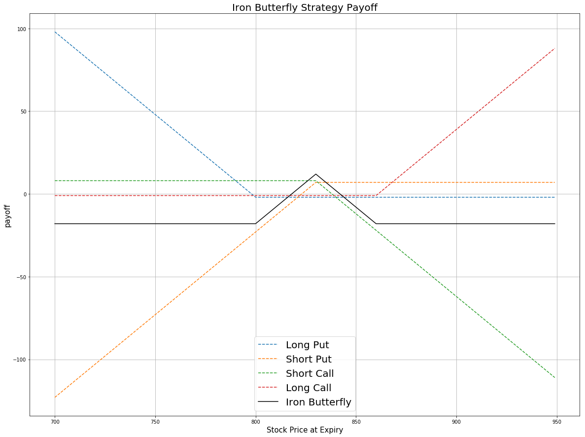
From the payoff plot, the maximum gain is simply the net credit you received when you buy and sell 4 options. This occurs if the stock price is exactly the same as the strike price of the ATM options. In this situation, all options expire worthless and you keep all premiums received. Although the Iron Butterfly has a narrower structure than the Iron Condor, the profit can be higher than with the Iron Condor as you receive a higher premium by selling ATM options than OTM options.

The maximum loss occurs if the underlying price is either below the OTM put strike or above the OTM call strike. In these two situations, two puts or two calls are exercised and the other two options expire worthless.

Implementation

Step 1: Initialize your algorithm by setting the start date, end date and the cash. Then, implement the coarse selection of the options contracts.

def Initialize(self):
    self.SetStartDate(2017, 2, 1)
    self.SetEndDate(2017, 3, 31)
    self.SetCash(300000)
    equity = self.AddEquity("GOOG", Resolution.Minute)
    option = self.AddOption("GOOG", Resolution.Minute)
    self.symbol = option.Symbol
    option.SetFilter(-10, 10, timedelta(0), timedelta(30))
    # use the underlying equity GOOG as the benchmark
    self.SetBenchmark(equity.Symbol)

Step 2: Break the candidate contracts into the call and put options.

def TradeOptions(self,optionchain):
    for i in optionchain:
        if i.Key != self.symbol: continue
    chain = i.Value
    # filter the call and put options from the contracts
    call = [i for i in chain if i.Right == 0]
    put = [i for i in chain if i.Right == 1]

Step 3: Sort the call and put options according to their strike prices. option.SetFilter(-10, 10, 0, 30) helps us choose 21 call options and 21 put options which expire within 30 days from now. Then for the call options, the first 10 contracts are in the money and the last 10 contracts are out of the money. The middle one is an at the money option. For the put options, the first 10 contracts are out of the money and the last 10 contracts are in the money.

call_contracts = sorted(call,key = lambda x: x.Strike)
put_contracts = sorted(put,key = lambda x: x.Strike)
if len(call_contracts) == 0 or len(put_contracts) == 0 : continue

Step 4: Find the specific contracts to trade. At the money options have the minimum absolute difference between the underlying price and the strike price.

# Sell 1 ATM Put
self.atm_put = sorted(put_contracts,key = lambda x: abs(chain.Underlying.Price - x.Strike))[0]
self.Sell(self.atm_put.Symbol ,1)
# Sell 1 ATM Call
self.atm_call = sorted(call_contracts,key = lambda x: abs(chain.Underlying.Price - x.Strike))[0]
self.Sell(self.atm_call.Symbol ,1)
# Buy 1 OTM Call
self.otm_call = call_contracts[-1]
self.Buy(self.otm_call.Symbol ,1)
# Buy 1 OTM Put
self.otm_put = put_contracts[0]
self.Buy(self.otm_put.Symbol ,1)

Summary

In this algorithm, on 04/03/2017, the share price of Google is $832.8. We buy OTM put(strike = $805) at $2, OTM call(strike = $860) and sell an ATM call and an ATM put. At the expiry 04/21/2017, the share price is $841.53. The ATM call is exercised and the other 3 options expire worthless. As we hold the short position of the ATM call, after expiration we will be short 100 shares of GOOG.

---

---

---