Hey everyone,In this post, I'm going to do my best to concisely explain what LSTM neural networks are and give an example of how to use them in your algorithm. If you want more information on LSTM, I highly recommend reading this post on how LSTM operates.

Recurrent neural networks (RNN) are an extremely powerful tool in deep learning. These models quite accurately mimic how humans process information and learn. Unlike traditional feedforward neural networks, RNNs have memory. That is, information fed into them persists and the network is able to draw on this to make inferences. In traditional neural networks, data is fed into the network and an output is produced. However, RNNs feed some information back into itself -- it decides to remember certain things rather than scraping all previous data. This functionality is massively powerful and has led to amazing achievements, but there is also a serious problem that accompanies RNNs -- the vanishing gradient.The vanishing gradient problem is essentially the inability of RNNs to handle long-term data dependencies. In neutral networks, gradients are found using backpropagation, which computes the gradient of the loss function with respect to the weights of the network. In backpropagation, the derivatives of each layer are multiplied down the network (from the final layer to the initial) to compute the derivatives of the initial layers. As more layers are added to the network, the chain-rule for derivatives means that small derivatives can compound quickly and the gradients of the loss function can approach zero. Such small gradients mean that the input weights for the initial layers can be so small that data is no longer recognized, effectively preventing the network from continuing to train.The solution to this problem is long short-term memory (LSTM), a type of recurrent neural network. Instead of one layer, LSTM cells generally have four, three of which are part of "gates" -- ways to optionally let information through. The three gates are commonly referred to as the forget, input, and output gates. The forget gate layer is where the model decides what information to keep from prior states. At the input gate layer, the model decides which values to update. Finally, the output gate layer is where the final output of the cell state is decided. Essentially, LSTM separately decides what to remember and the rate at which it should update. There is a lot of work that goes on behind the scenes here and this is just the broad strokes of what happens, but the essential difference between LSTM and n naive RNN is that LSTM is better equipped at handling long-term memory and avoids the vanishing gradient problem.

LSTM has been applied to fields as diverse as speech recognition, text recognition and translation, image processing, and robotic control. In addition to these fields, LSTM models have produced some great results when applied to time-series prediction. One of the central challenges with conventional time-series models is that, despite trying to account for trends or other non-stationary elements, it is almost impossible to truly predict an outlier like a recession, flash crash, liquidity crisis, etc. By having a long memory, LSTM models are better able to capture these difficult trends in the data without suffering from the level of overfitting a conventional model would need in order to capture the same data.

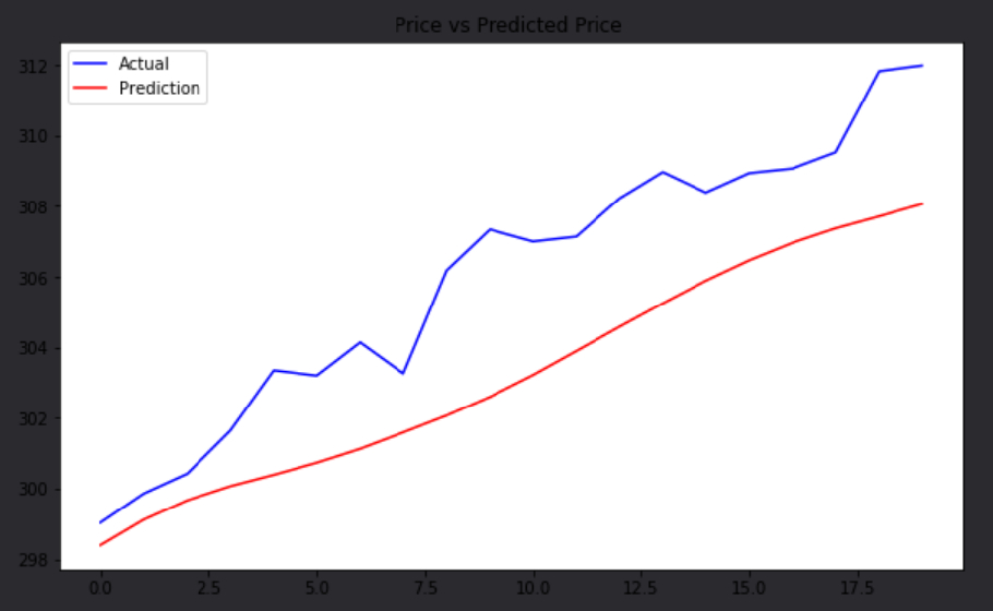
For a very basic application, we're going to use an LSTM model to predict the price movement, a non-stationary time-series, of SPY (the structure of the model setup below was adapted from this post). In the research notebook, we ran the following code:

import numpy as np
import pandas as pd
import matplotlib.pyplot as plt
from sklearn.preprocessing import MinMaxScaler
qb = QuantBook() 
symbol = qb.AddEquity("SPY").Symbol 
# Fetch history history = qb.History([symbol], 1280, Resolution.Daily) 
# Fetch price 
total_price = history.loc[symbol].close 
training_price = history.loc[symbol].close[:1260] 
test_price = history.loc[symbol].close[1260:] 
# Transform price 
price_array = np.array(training_price).reshape((len(training_price), 1) 
# Import keras modules 
from keras.layers import LSTM 
from keras.layers import Dense 
from keras.layers import Dropout 
from keras.models import Sequential 
# Build a Sequential keras model 
model = Sequential() 
# Add our first LSTM layer - 50 nodes 
model.add(LSTM(units = 50, return_sequences=True, input_shape=(features_set.shape[1], 1))) 
# Add Dropout layer to avoid overfitting 
model.add(Dropout(0.2)) 
# Add additional layers 
model.add(LSTM(units=50, return_sequences=True)) 
model.add(Dropout(0.2)) 
model.add(LSTM(units=50, return_sequences=True)) 
model.add(Dropout(0.2)) model.add(LSTM(units=50)) 
model.add(Dropout(0.2)) model.add(Dense(units = 1)) 
# Compile the model 
model.compile(optimizer = 'adam', loss = 'mean_squared_error', metrics=['mae', 'acc']) 
# Fit the model to our data, running 100 training epochs 
model.fit(features_set, labels, epochs = 50, batch_size = 32) 
# Get and transform inputs for testing our predictions 
test_inputs = total_price[-80:].values 
test_inputs = test_inputs.reshape(-1,1) 
test_inputs = scaler.transform(test_inputs) 
# Get test features 
test_features = [] for i in range(60, 80): 
test_features.append(test_inputs[i-60:i, 0]) 
test_features = np.array(test_features) 
test_features = np.reshape(test_features, (test_features.shape[0], test_features.shape[1], 1)) 
# Make predictions 
predictions = model.predict(test_features) 
# Transform predictions back to original data-scale 
predictions = scaler.inverse_transform(predictions) 
# Plot our results! 
plt.figure(figsize=(10,6)) 
plt.plot(test_price.values, color='blue', label='Actual') 
plt.plot(predictions , color='red', label='Prediction') 
plt.title('Price vs Predicted Price ') 
plt.legend() 
plt.show() 
# In Initialize 
self.Train(self.DateRules.MonthEnd(), self.TimeRules.At(8,0), self.TrainMyModel) 
def TrainMyModel(self): 
    qb = self 
    # Fetch history 
    history = qb.History([symbol for key, symbol in self.macro_symbols.items()], 1280, Resolution.Daily) 
    # Iterate over macro symbols 
    for key, symbol in self.macro_symbols.items(): 
        # Initialize LSTM class instance 
        lstm = MyLSTM() 
        # Prepare data 
        features_set, labels, training_data, test_data = lstm.ProcessData(history.loc[symbol].close) 
        # Build model layers 
        lstm.CreateModel(features_set, labels) 
        # Fit model 
        lstm.FitModel(features_set, labels) 
        # Add LSTM class to dictionary to store later 
        self.models[key] = lstm
+ Expand
- Collapse

The algorithm we built to demonstrate how LSTM can be incorporated into QuantConnect is very simple. We used the model from the research environment and predicted the next price of SPY each day. Then, we emit Insights for inverse Treasury ETFs and SP500 Sector ETFs if the prediction is up, and we emit Insights for long Treasury ETFs if not. To do this we broke the algorithm up into a few methods. First, we built a scheduled event to train the model every month. Since this is a computationally-intensive operation, we wrapped the scheduled event in the Train() method.

# In Initialize 
self.Train(self.DateRules.MonthEnd(), self.TimeRules.At(8,0), self.TrainMyModel) 
def TrainMyModel(self): 
    qb = self 
    # Fetch history 
    history = qb.History([symbol for key, symbol in self.macro_symbols.items()], 1280, Resolution.Daily) 
    # Iterate over macro symbols 
    for key, symbol in self.macro_symbols.items(): 
        # Initialize LSTM class instance lstm = MyLSTM() 
        # Prepare data 
        features_set, labels, training_data, test_data = lstm.ProcessData(history.loc[symbol].close) 
        # Build model layers lstm.CreateModel(features_set, labels) 
        # Fit model 
        lstm.FitModel(features_set, labels) 
        # Add LSTM class to dictionary to store later 
        self.models[key] = lstm
+ Expand
- Collapse

Then, we built a predict function to make our predictions every day, 5-minutes after MarketOpen.

def Predict(self): delta = {} qb = self for key, symbol in self.macro_symbols.items(): # Fetch LSTM class lstm = self.models[key] # Fetch history history = qb.History([symbol for key, symbol in self.macro_symbols.items()], 80, Resolution.Daily) # Predict predictions = lstm.PredictFromModel(history.loc[symbol].close) # Grab latest prediction and calculate if predict symbol to go up or down delta[key] = ( predictions[-1] / self.Securities[symbol].Price ) - 1 # Plot prediction self.Plot('Prediction Plot', f'Predicted {key}', predictions[-1]) insights = [] # Iterate over macro symbols for key, change in delta.items(): if key == 'Bull': insights += [Insight.Price(symbol, timedelta(1), InsightDirection.Up if change > 0 else InsightDirection.Flat) for symbol in LiquidETFUniverse.SP500Sectors.Long if self.Securities.ContainsKey(symbol)] insights += [Insight.Price(symbol, timedelta(1), InsightDirection.Up if change > 0 else InsightDirection.Flat) for symbol in LiquidETFUniverse.Treasuries.Inverse if self.Securities.ContainsKey(symbol)] insights += [Insight.Price(symbol, timedelta(1), InsightDirection.Flat if change > 0 else InsightDirection.Up) for symbol in LiquidETFUniverse.Treasuries.Long if self.Securities.ContainsKey(symbol)] self.EmitInsights(insights)

Finally, we added a short method to plot the actual price vs the predicted price, which allows us to visually track what was happening in the algorithm.

def PlotMe(self): # Plot current price of symbols to match against prediction for key, symbol in self.macro_symbols.items(): self.Plot('Prediction Plot', f'Actual {key}', self.Securities[symbol].Price)

Since this is a computationally expensive algorithm, we used the Train() method, which allows for extended model-training without throwing a timeout error. This will be extremely useful for anyone looking to add ML methods to their algorithms, and you can find another example of this method here.Once the backtest runs, you can see that the model's predictions are fairly accurate considering the difficulties associated with modeling and predicting from a non-stationary series. It's not close enough for us to be able to claim to know the next SPY price at any given time, but it clearly gives sufficient information to inform us about market conditions at-large.